Chapter 2 Introduction to NEON & its Data
Estimated Time: 2 hours
Course participants: As you review this information, please consider the final course project that you will work on the over this semester. At the end of this section you will document an initial research question, or idea and associated data needed to address that question, that you may want to explore while pursuing this course.
2.1 Learning Objectives
At the end of this activity, you will be able to:
- Explain the mission of the National Ecological Observatory Network (NEON).
- Explain the how sites are located within the NEON project design.
- Determine how the different types of data that are collected and provided by NEON, and how they align with your own research.
- Pull NEON data from the API and
neonUtilitiespackage [@R-neonUtilites]
2.2 The NEON Project Mission & Design
To capture ecological heterogeneity across the United States, NEON’s design divides the continent into 20 statistically different eco-climatic domains. Each NEON field site is located within an eco-climatic domain.
2.3 The Science and Design of NEON
To gain a better understanding of the broad scope of NEON watch this 4:08 minute long video.
2.4 NEON’s Spatial Design
Watch this 4:22 minute video exploring the spatial design of NEON field sites.
Please read the following page about NEON’s Spatial Design:
2.4.1 NEON Samples All 20 Eco-Regions
Explore the NEON Field Site map taking note of the locations of:
- Aquatic & terrestrial field sites.
- Core & relocatable field sites.
Click here to view the NEON Field Site Map
Explore the NEON field site map. Do the following:
- Zoom in on a study area of interest to see if there are any NEON field sites that are nearby.
- Click the “More” button in the upper right hand corner of the map to filter sites by name, site host, domain or state.
- Select one field site of interest.
- Click on the marker in the map.
- Then click on the name of the field site to jump to the field site landing page.
Data Tip: You can download maps, kmz, or shapefiles of the field sites here.
2.5 How NEON Collects Data
Watch this 3:06 minute video exploring the data that NEON collects.
Read the Data Collection Methods page to learn more about the different types of data that NEON collects and provides. Then, follow the links below to learn more about each collection method:
- Aquatic Observation System (AOS)
- Aquatic Instrument System (AIS)
- Terrestrial Instrument System (TIS) – Flux Tower
- Terrestrial Instrument System (TIS) – Soil Sensors and Measurements
- Terrestrial Organismal System (TOS)
- Airborne Observation Platform (AOP)
All data collection protocols and processing documents are publicly available. Read more about the standardized protocols and how to access these documents.
2.5.1 Specimens & Samples
NEON also collects samples and specimens from which the other data products are based. These samples are also available for research and education purposes. Learn more: NEON Biorepository.
2.5.2 Airborne Remote Sensing
Watch this 4:02 minute video to better understand the NEON Airborne Observation Platform (AOP).
Data Tip: NEON also provides support to your own research including proposals to fly the AOP over other study sites, a mobile tower/instrumentation setup and others. Learn more here the Assignable Assets programs .
2.6 Accessing NEON Data
NEON data are processed and go through quality assurance quality control checks at NEON headquarters in Boulder, CO. NEON carefully documents every aspect of sampling design, data collection, processing and delivery. This documentation is freely available through the NEON data portal.
- Visit the NEON Data Portal - data.neonscience.org
- Read more about the quality assurance and quality control processes for NEON data and how the data are processed from raw data to higher level data products.
- Explore NEON Data Products. On the page for each data product in the catalog you can find the basic information about the product, find the data collection and processing protocols, and link directly to downloading the data.
- Additionally, some types of NEON data are also available through the data portals of other organizations. For example, NEON Terrestrial Insect DNA Barcoding Data is available through the Barcode of Life Datasystem (BOLD). Or NEON phenocam images are available from the Phenocam network site. More details on where else the data are available from can be found in the Availability and Download section on the Product Details page for each data product (visit Explore Data Products to access individual Product Details pages).
2.6.1 Pathways to access NEON Data
There are several ways to access data from NEON:
- Via the NEON data portal.
Explore and download data. Note that much of the tabular data is available in zipped
.csv files for each month and site of interest. To combine these files, use the
neonUtilities package (R tutorial, Python tutorial).
- Use R or Python to programmatically access the data. NEON and community members
have created code packages to directly access the data through an API. Learn more
about the available resources by reading the Code Resources page or visiting the
NEONScience GitHub repo.
- Using the NEON API. Access NEON data directly using a custom API call.
- Access NEON data through partner’s portals. Where NEON data directly overlap with other community resources, NEON data can be accessed through the portals. Examples include Phenocam, BOLD, Ameriflux, and others. You can learn more in the documentation for individual data products.
2.7 Hands on: Accessing NEON Data & User Tokens
2.7.1 Via the NEON API, with your User Token
NEON data can be downloaded from either the NEON Data Portal or the NEON API. When downloading from the Data Portal, you can create a user account. Read about the benefits of an account on the User Account page. You can also use your account to create a token for using the API. Your token is unique to your account, so don’t share it.
While using a token is optional in general, it is required for this course. Using a token when downloading data via the API, including when using the neonUtilities package, links your downloads to your user account, as well as enabling faster download speeds. For more information about token usage and benefits, see the NEON API documentation page.
For now, in addition to faster downloads, using a token helps NEON to track data downloads. Using anonymized user information, they can then calculate data access statistics, such as which data products are downloaded most frequently, which data products are downloaded in groups by the same users, and how many users in total are downloading data. This information helps NEON to evaluate the growth and reach of the observatory, and to advocate for training activities, workshops, and software development.
Tokens can (and should) be used whenever you use the NEON API. In this tutorial, we’ll focus on using tokens with the neonUtilities R package.
2.7.1 Objectives
After completing this section, you will be able to:
- Create a NEON API token
- Use your token when downloading data with neonUtilities
2.7.1 Things You’ll Need To Complete This Tutorial
You will need a version of R (3.4.1 or higher) and RStudio
loaded on your computer.
2.7.1 Install R Packages
- neonUtilities:
install.packages("neonUtilities")
2.7.1 Additional Resources
If you’ve never downloaded NEON data using the neonUtilities package before, we recommend starting with the Download and Explore tutorial before proceeding with this tutorial.
In the next sections, we’ll get an API token from the NEON Data Portal, and then use it in neonUtilities when downloading data.
2.7.2 Get a NEON API Token
The first step is create a NEON user account, if you don’t have one. Follow the instructions on the Data Portal User Accounts page. If you do already have an account, go to the NEON Data Portal, sign in, and go to your My Account profile page.
Once you have an account, you can create an API token for yourself. At the bottom of the My Account page, you should see this bar:

Click the ‘GET API TOKEN’ button. After a moment, you should see this:
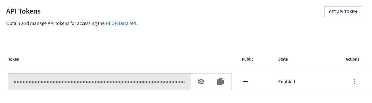
Click on the Copy button to copy your API token to the clipboard.
2.7.3 Use the API token in neonUtilities
In the next section, we’ll walk through saving your token somewhere secure but accessible to your code. But first let’s try out using the token the easy way.
First, we need to load the neonUtilities package and set the working
directory:
# install neonUtilities - can skip if already installed, but
# API tokens are only enabled in neonUtilities v1.3.4 and higher
# if your version number is lower, re-install
install.packages("neonUtilities")
# load neonUtilities
library(neonUtilities)
# set working directory
wd <- "~/data" # this will depend on your local machine
setwd(wd)
NEON API tokens are very long, so it would be annoying to keep pasting the entire text string into functions. Assign your token an object name:
Now we’ll use the loadByProduct() function to download data. Your
API token is entered as the optional token input parameter. For
this example, we’ll download Plant foliar traits (DP1.10026.001).
foliar <- loadByProduct(dpID="DP1.10026.001", site="all",
                        package="expanded", check.size=F,
                        token=NEON_TOKEN)
You should now have data saved in the foliar object; the API
silently used your token. If you’ve downloaded data without a
token before, you may notice this is faster!
This format applies to all neonUtilities functions that involve
downloading data or otherwise accessing the API; you can use the
token input with all of them. For example, when downloading
remote sensing data:
2.7.4 Token management for open code
Your API token is unique to your account, so don’t share it!
If you’re writing code that will be shared with colleagues or available
publicly, such as in a GitHub repository or supplemental materials of a
published paper, you can’t include the line of code above where we assigned
your token to NEON_TOKEN, since your token is fully visible in the code
there. Instead, you’ll need to save your token locally on your computer,
and pull it into your code without displaying it. There are a few ways to
do this, we’ll show two options here.
Option 1: Save the token in a local file, and
source()that file at the start of every script. This is fairly simple but requires a line of code in every script.Option 2: Add the token to a
.Renvironfile to create an environment variable that gets loaded when you open R. This is a little harder to set up initially, but once it’s done, it’s done globally, and it will work in every script you run.
2.7.4.1 Option 1: Save token in a local file
Open a new, empty R script (.R). Put a single line of code in the script:
Save this file within your current R project and call the file neon_token_source.R. So that you don’t accidently push your token up to GitHub, move over to the command line or Atom.io and add it to your .gitignore file:
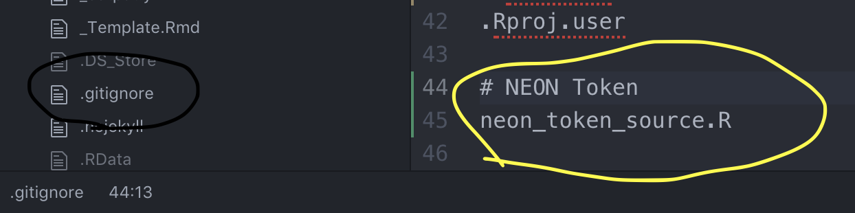
Now, whenever you want to pull NEON data via the API, at the start of any analysis you would place this line of code:
Then you’ll be able to use token=NEON_TOKEN when you run neonUtilities
functions, and you can share your code without accidentally sharing your
token.
2.7.4.2 Option 2: Save your toekn to your R environment
Instructions for finding and editing your .Renviron can be found in this tutorial in NEON’s Data Tutorials section.
2.8 Hands on: NEON TOS Data
2.8.1 Pull in Tree Data from NEON’s TOS and investigate relationships
Adapted from Claire Lunch’s ‘Compare tree height measured from the ground to a Lidar-based Canopy Height Model’ tutorial
Later in this course we will be working with NEON’s LiDAR-based Canopy Height Model (CHM) data from their extensive Airborne Observation Platform (AOP). In this section we will pull in DP1.10098.001, Woody plant vegetation structure from NEON’s Terrestrial Observation Sampling (TOS) data and explore the data, from requesting it to plotting it.
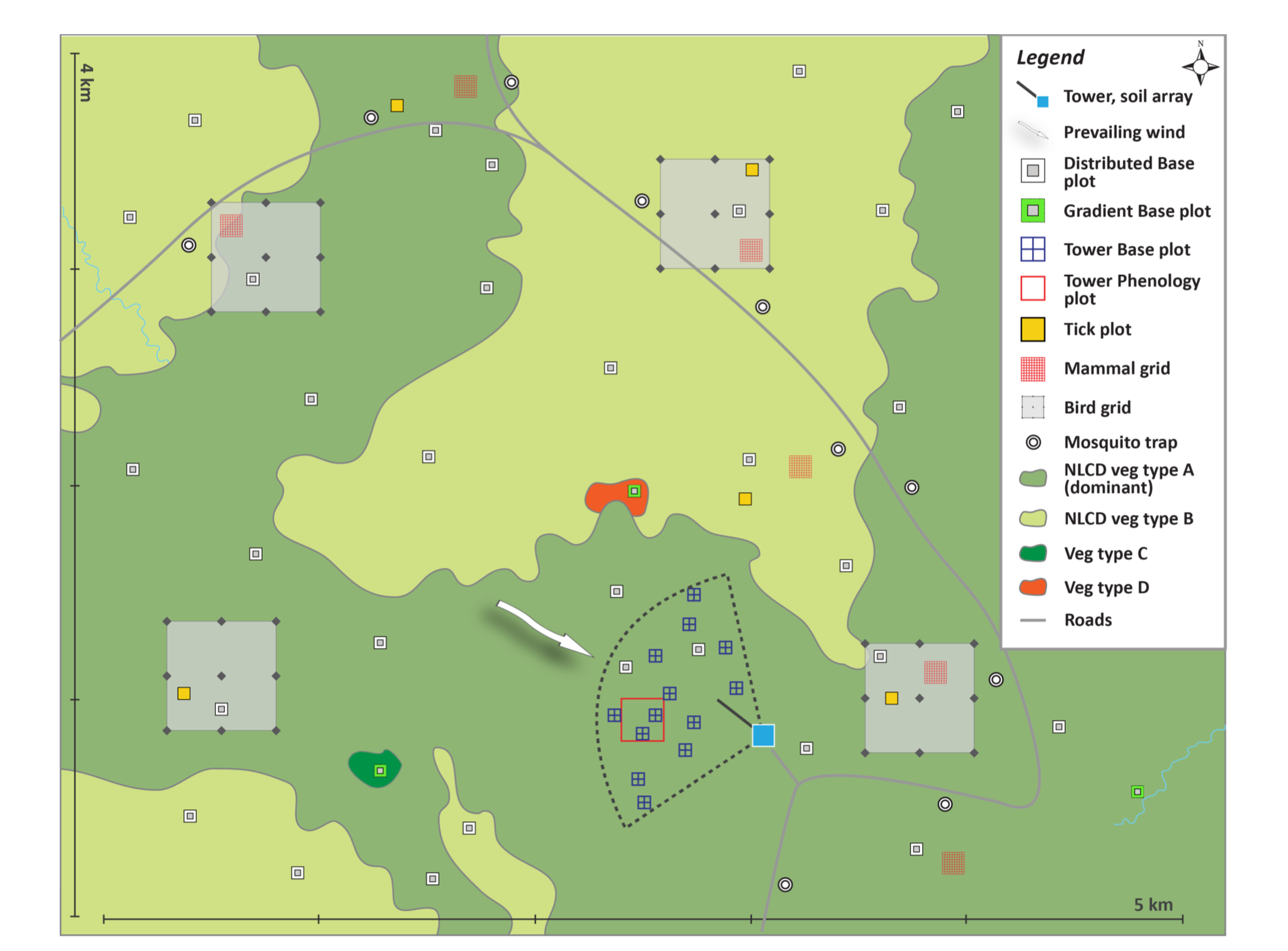
Generalized TOS sampling schematic, showing the placement of Distributed, Tower, and Gradient Plots from the NEON GUIDE TO WOODY PLANT VEGETATION STRUCTURE, 2018
The vegetation structure data are collected by by field staff on the ground. This data product contains the quality-controlled, native sampling resolution data from in-situ measurements of live and standing dead woody individuals and shrub groups, from all terrestrial NEON sites with qualifying woody vegetation. The exact measurements collected per individual depend on growth form, and these measurements are focused on enabling biomass and productivity estimation, estimation of shrub volume and biomass, and calibration / validation of multiple NEON airborne remote-sensing data products. In general, comparatively large individuals that are visible to remote-sensing instruments are mapped, tagged and measured, and other smaller individuals are tagged and measured but not mapped. Smaller individuals may be subsampled according to a nested subplot approach in order to standardize the per plot sampling effort. Structure and mapping data are reported per individual per plot; sampling metadata, such as per growth form sampling area, are reported per plot.
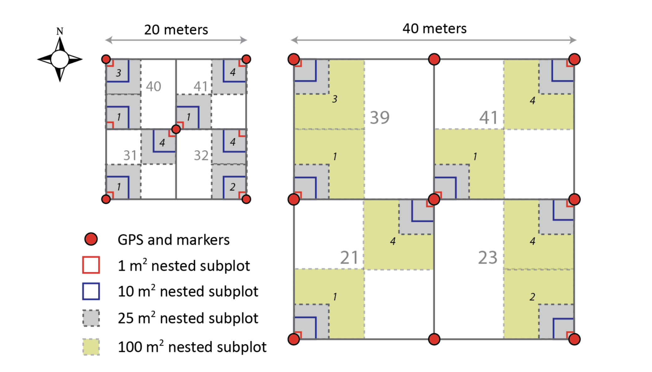
Illustration of a 20 m x 20 m Distributed/Gradient/Tower base plot (left), a 40 m x 40 m Tower base plot (right), and associated nested subplots used for measuring woody stem vegetation. Locations of subplots are denoted with plain text numbers, and locations of nested subplots are denoted with italic numbers from the NEON GUIDE TO WOODY PLANT VEGETATION STRUCTURE, 2018
For the purpose of this hands-on activity we will be using data from the Wind River Experimental Forest NEON field site located in Washington state. The predominant vegetation at that site is tall evergreen conifers.
Note: this is also a core site for many other networks such as AmeriFlux and FLUXNET, which we will cover later.
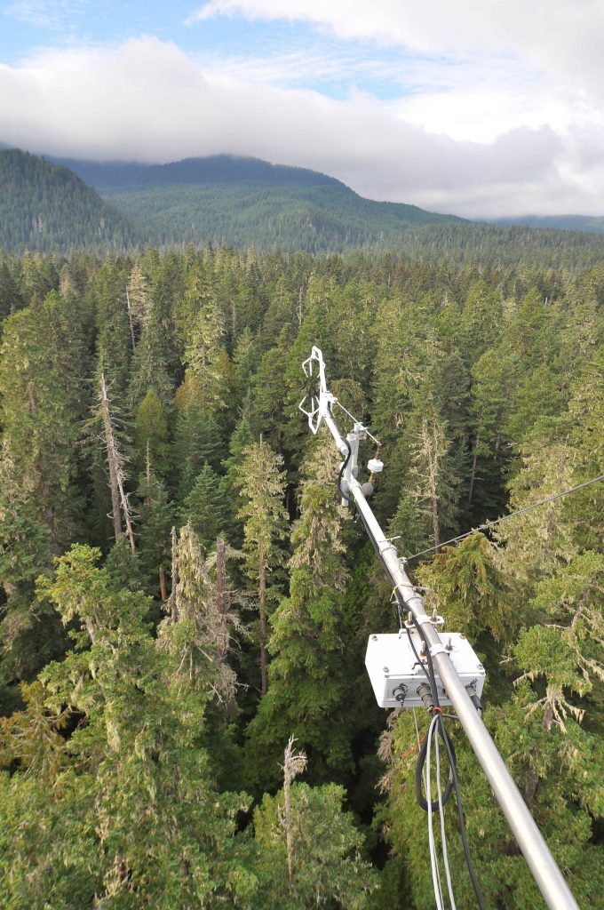
Image of the Wind River Crane Flux Tower from Ameriflux
Let’s begin by:
- Installing the
geoNEONpackage - Making sure that the packages that we need are loaded, and
- Supressing ‘strings as factors’ in R, as factors make all sorts of functions in R ‘cranky’.
options(stringsAsFactors=F)

#install.packages("devtools") #uncomment if you don't yet have devtools
#devtools::install_github("NEONScience/NEON-geolocation/geoNEON")

library(neonUtilities)
## Warning: package 'neonUtilities' was built under R version 3.6.2## Warning: package 'sp' was built under R version 3.6.2Now lets begin by pulling in the vegetation structure data using the loadByProduct() function in the neonUtilities package. Inputs needed to the function are:
dpID: data product ID; (woody vegetation structure = DP1.10098.001
site: 4-letter site code; Wind River = WREF
package: basic or expanded; we’ll begin with a
basichere
## Finding available files
##
  |
  |                                                                      |   0%
  |
  |=======================                                               |  33%
  |
  |===============================================                       |  67%
  |
  |======================================================================| 100%
##
## Downloading files totaling approximately 518.3 KiB
## Downloading 3 files
##
  |
  |                                                                      |   0%
  |
  |===================================                                   |  50%
  |
  |======================================================================| 100%
##
## Unpacking zip files using 1 cores.
## Stacking operation across a single core.
## Stacking table vst_apparentindividual
## Stacking table vst_mappingandtagging
## Stacking table vst_perplotperyear
## Copied the most recent publication of validation file to /stackedFiles
## Copied the most recent publication of categoricalCodes file to /stackedFiles
## Copied the most recent publication of variable definition file to /stackedFiles
## Finished: Stacked 3 data tables and 3 metadata tables!
## Stacking took 0.4544132 secs
## All unzipped monthly data folders have been removed.
Now, use the getLocTOS() function in the geoNEON package to get precise locations for the tagged plants. You can refer to the package documentation for more details.
##
|
| | 0%
|
| | 1%
|
|= | 1%
|
|= | 2%
|
|== | 2%
|
|== | 3%
|
|=== | 4%
|
|=== | 5%
|
|==== | 5%
|
|==== | 6%
|
|===== | 7%
|
|====== | 8%
|
|====== | 9%
|
|======= | 10%
|
|======== | 11%
|
|======== | 12%
|
|========= | 13%
|
|========== | 14%
|
|========== | 15%
|
|=========== | 16%
|
|============ | 17%
|
|============ | 18%
|
|============= | 18%
|
|============= | 19%
|
|============== | 20%
|
|============== | 21%
|
|=============== | 21%
|
|=============== | 22%
|
|================ | 22%
|
|================ | 23%
|
|================ | 24%
|
|================= | 24%
|
|================= | 25%
|
|================== | 25%
|
|================== | 26%
|
|=================== | 26%
|
|=================== | 27%
|
|=================== | 28%
|
|==================== | 28%
|
|==================== | 29%
|
|===================== | 29%
|
|===================== | 30%
|
|====================== | 31%
|
|====================== | 32%
|
|======================= | 32%
|
|======================= | 33%
|
|======================== | 34%
|
|========================= | 35%
|
|========================= | 36%
|
|========================== | 37%
|
|=========================== | 38%
|
|=========================== | 39%
|
|============================ | 40%
|
|============================= | 41%
|
|============================= | 42%
|
|============================== | 43%
|
|=============================== | 44%
|
|=============================== | 45%
|
|================================ | 45%
|
|================================ | 46%
|
|================================= | 47%
|
|================================= | 48%
|
|================================== | 48%
|
|================================== | 49%
|
|=================================== | 49%
|
|=================================== | 50%
|
|=================================== | 51%
|
|==================================== | 51%
|
|==================================== | 52%
|
|===================================== | 52%
|
|===================================== | 53%
|
|====================================== | 54%
|
|====================================== | 55%
|
|======================================= | 55%
|
|======================================= | 56%
|
|======================================== | 57%
|
|========================================= | 58%
|
|========================================= | 59%
|
|========================================== | 60%
|
|=========================================== | 61%
|
|=========================================== | 62%
|
|============================================ | 63%
|
|============================================= | 64%
|
|============================================= | 65%
|
|============================================== | 66%
|
|=============================================== | 67%
|
|=============================================== | 68%
|
|================================================ | 68%
|
|================================================ | 69%
|
|================================================= | 70%
|
|================================================= | 71%
|
|================================================== | 71%
|
|================================================== | 72%
|
|=================================================== | 72%
|
|=================================================== | 73%
|
|=================================================== | 74%
|
|==================================================== | 74%
|
|==================================================== | 75%
|
|===================================================== | 75%
|
|===================================================== | 76%
|
|====================================================== | 76%
|
|====================================================== | 77%
|
|====================================================== | 78%
|
|======================================================= | 78%
|
|======================================================= | 79%
|
|======================================================== | 79%
|
|======================================================== | 80%
|
|========================================================= | 81%
|
|========================================================= | 82%
|
|========================================================== | 82%
|
|========================================================== | 83%
|
|=========================================================== | 84%
|
|============================================================ | 85%
|
|============================================================ | 86%
|
|============================================================= | 87%
|
|============================================================== | 88%
|
|============================================================== | 89%
|
|=============================================================== | 90%
|
|================================================================ | 91%
|
|================================================================ | 92%
|
|================================================================= | 93%
|
|================================================================== | 94%
|
|================================================================== | 95%
|
|=================================================================== | 95%
|
|=================================================================== | 96%
|
|==================================================================== | 97%
|
|==================================================================== | 98%
|
|===================================================================== | 98%
|
|===================================================================== | 99%
|
|======================================================================| 99%
|
|======================================================================| 100%Now we need to merge the mapped locations of individuals (the vst_mappingandtagging table) with the annual measurements of height, diameter, etc (the vst_apparentindividual table). The two tables join based on individualID, the identifier for each tagged plant, but we’ll include namedLocation, domainID, siteID, and plotID in the list of variables to merge on, to avoid ending up with duplicates of each of those columns. Refer to the variables table and to the Data Product User Guide for Woody plant vegetation structure for more information about the contents of each data table.
veg <- merge(veglist$vst_apparentindividual, vegmap,
             by=c("individualID","namedLocation",
                  "domainID","siteID","plotID"))
What did you just pull in? Are you sure you know what you’re working with? A best practice is to always do a quick visualization to make sure that you have the right data and that you understand its spread:
symbols(veg$adjEasting[which(veg$plotID=="WREF_075")],
        veg$adjNorthing[which(veg$plotID=="WREF_075")],
        circles=veg$stemDiameter[which(veg$plotID=="WREF_075")]/100/2,
        inches=F, xlab="Easting", ylab="Northing")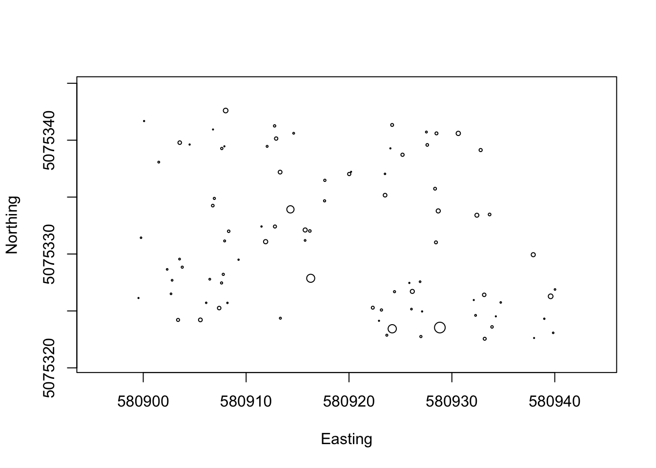
A key component of any measurement, and therefore a reoccuring theme in this course, is an estimate of uncertainty. Let’s overlay estimates of uncertainty for the location of each stem in blue:
symbols(veg$adjEasting[which(veg$plotID=="WREF_075")],
        veg$adjNorthing[which(veg$plotID=="WREF_075")],
        circles=veg$stemDiameter[which(veg$plotID=="WREF_075")]/100/2,
        inches=F, xlab="Easting", ylab="Northing")
symbols(veg$adjEasting[which(veg$plotID=="WREF_075")],
        veg$adjNorthing[which(veg$plotID=="WREF_075")],
        circles=veg$adjCoordinateUncertainty[which(veg$plotID=="WREF_075")],
        inches=F, add=T, fg="lightblue")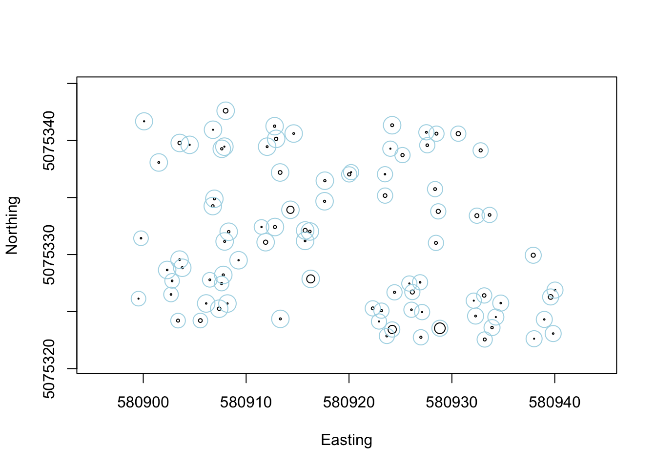
2.9 Intro to NEON Exercises Part 1
2.9.1 Computational
2.9.1.1 Part 1: Sign up for and Use an NEON API Token:
- Submit via .Rmd and .pdf a simple script that uses a HIDDEN token to access NEON data.
Example:
source('neon_token_source.R')
veglist <- loadByProduct(dpID="DP1.10098.001", site="WREF", package="basic", check.size=FALSE, token = NEON_TOKEN)
## Finding available files
##
|
| | 0%
|
|======================= | 33%
|
|=============================================== | 67%
|
|======================================================================| 100%
##
## Downloading files totaling approximately 518.3 KiB
## Downloading 3 files
##
|
| | 0%
|
|=================================== | 50%
|
|======================================================================| 100%
##
## Unpacking zip files using 1 cores.
## Stacking operation across a single core.
## Stacking table vst_apparentindividual
## Stacking table vst_mappingandtagging
## Stacking table vst_perplotperyear
## Copied the most recent publication of validation file to /stackedFiles
## Copied the most recent publication of categoricalCodes file to /stackedFiles
## Copied the most recent publication of variable definition file to /stackedFiles
## Finished: Stacked 3 data tables and 3 metadata tables!
## Stacking took 0.146975 secs
## All unzipped monthly data folders have been removed.## Length Class Mode
## categoricalCodes_10098 5 data.table list
## readme_10098 1 spec_tbl_df list
## validation_10098 8 data.table list
## variables_10098 9 data.table list
## vst_apparentindividual 40 data.frame list
## vst_mappingandtagging 29 data.frame list
## vst_perplotperyear 38 data.frame list2.9.1.2 Part 2: Further Investigation of NEON TOS Vegetation Structure Data
Suggested Timing: Complete this exercise before our next class session
In the following section all demonstration code uses the iris dataset for R as examples. In this exercise the iris data is merely used for example code to get your started, you will complete all plots and models using the NEON TOS vegetation structure data
- Convert the above diameter plot into a ggplot: If you need some refreshers on ggplot Derek Sonderegger’s Introductory Data Science using R: Graphing Part II is a wonderful resource. I’ve pulled some of his plotting examples here.
## Warning: package 'ggplot2' was built under R version 3.6.2## [1] "your code here"- Set the color your circles to be a function of each species:
#hints:
data("iris")
ggplot(iris, aes(x=Sepal.Length, y=Petal.Length, color=Species)) +
geom_point() 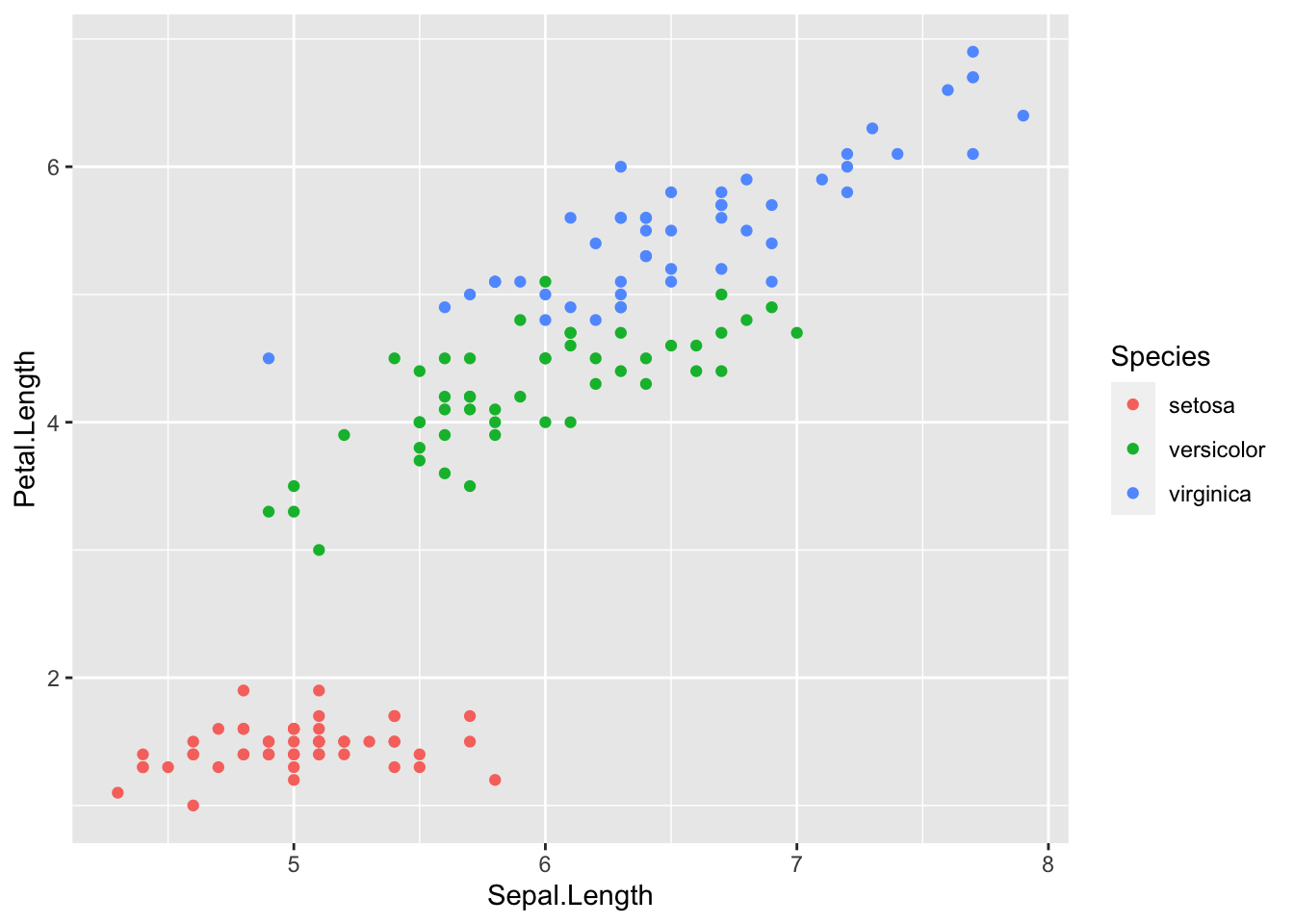
- Generate a histogram of tree heights for each plot. Color your stacked bar as a function of each species:
#hints for faceting:
ggplot(iris, aes(x=Sepal.Length, y=Petal.Length)) +
  geom_point() +
  facet_grid( . ~ Species )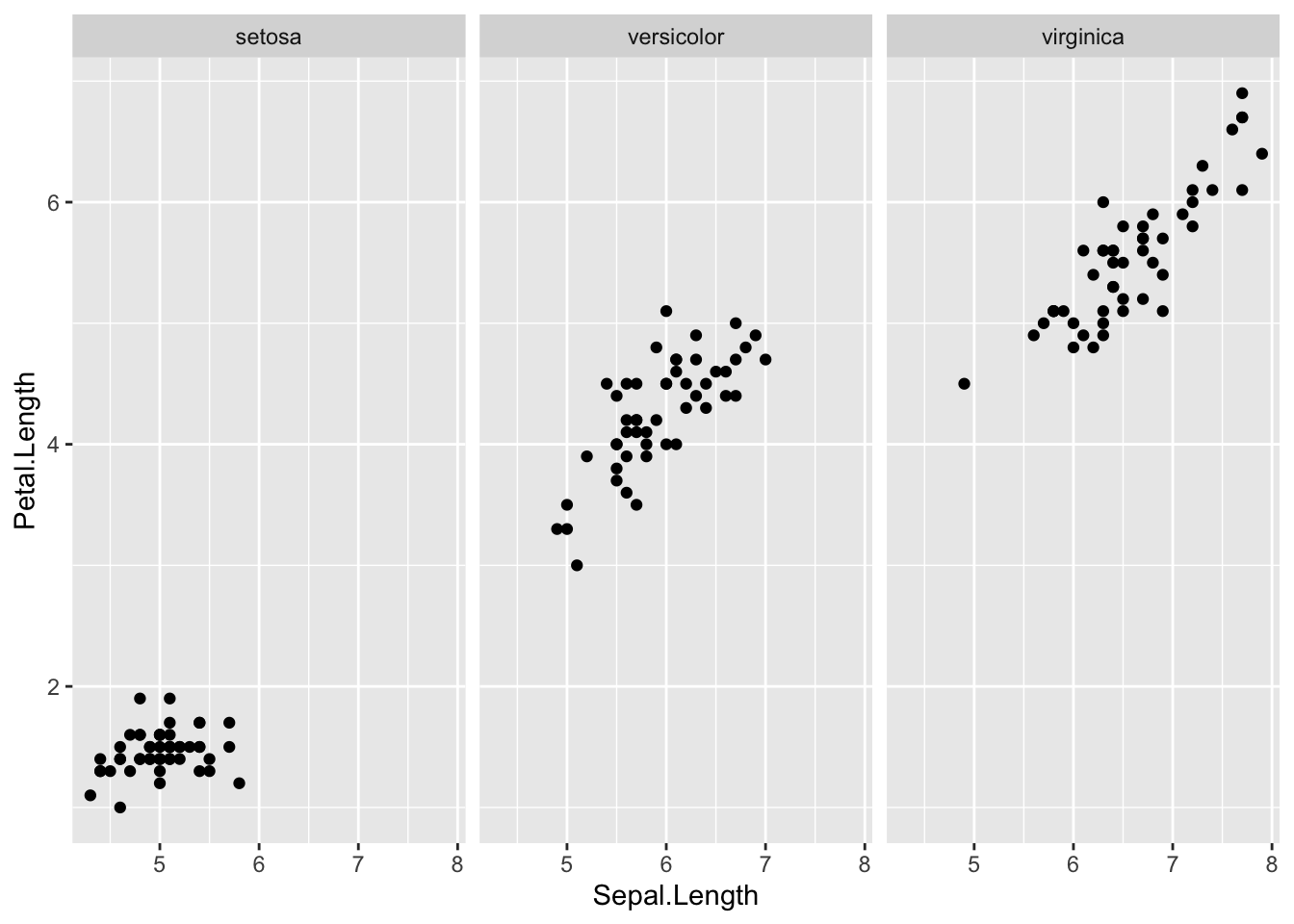
- Use
dplyrto remove dead trees:
## Warning: package 'dplyr' was built under R version 3.6.2##
## Attaching package: 'dplyr'## The following objects are masked from 'package:stats':
##
## filter, lag## The following objects are masked from 'package:base':
##
## intersect, setdiff, setequal, union- Create a simple linear model that uses Diameter at Breast Height (DBH) and height to predict allometries. Print the summary information of your model:
#hints
mdl=lm(Some_diameter + Some_height, data=something) #Question: looking at the metadata which 'height' and 'diameter' variables should you use?
print(mdl)- Plot your linear model:
# hints:
mdl <- lm( Petal.Length ~ Sepal.Length * Species, data = iris )
iris <- iris %>%
  select( -matches('fit'), -matches('lwr'), -matches('upr') ) %>%
  cbind( predict(mdl, newdata=., interval='confidence') )

head(iris, n=3)
## Sepal.Length Sepal.Width Petal.Length Petal.Width Species fit lwr
## 1 5.1 3.5 1.4 0.2 setosa 1.474373 1.398783
## 2 4.9 3.0 1.4 0.2 setosa 1.448047 1.371765
## 3 4.7 3.2 1.3 0.2 setosa 1.421721 1.324643
## upr
## 1 1.549964
## 2 1.524329
## 3 1.518798ggplot(iris, aes(x=Sepal.Length, y=Petal.Length, color=Species)) +
geom_point() +
geom_line( aes(y=fit) ) +
geom_ribbon( aes( ymin=lwr, ymax=upr, fill=Species), alpha=.3 ) # alpha is the ribbon transparency
- Answer the following questions:
- What do you think about your simile linear model? What are its limitations?
- How many
uniquespecies are present atWREF? - What are the
top_5trees based on height? Diameter? - What proportion of sampled trees are dead?
2.10 Part 2: Pulling NEON Data via the API
This section covers pulling data from the NEON API or Application Programming Interface using R and the R package httr, but the core information about the API is applicable to other languages and approaches.
As a reminder, there are 3 basic categories of NEON data:
- Observational - Data collected by a human in the field, or in an analytical laboratory, e.g. beetle identification, foliar isotopes
- Instrumentation - Data collected by an automated, streaming sensor, e.g. net radiation, soil carbon dioxide
- Remote sensing - Data collected by the airborne observation platform, e.g. LIDAR, surface reflectance
This lab covers all three types of data, it is required to complete these sections in order and not skip ahead, since the query principles are explained in the first section, on observational data.
2.10 Objectives
After completing this activity, you will be able to:
- Pull observational, instrumentation, and geolocation data from the NEON API.
- Transform API-accessed data from JSON to tabular format for analyses.
2.10 Things You’ll Need To Complete This Section
To complete this tutorial you will need the most current version of R and, preferably, RStudio loaded on your computer.
2.10 Install R Packages
- httr:
install.packages("httr") - jsonlite:
install.packages("jsonlite") - dplyr:
install.packages("dplyr") - devtools:
install.packages("devtools") - downloader:
install.packages("downloader") - geoNEON:
devtools::install_github("NEONScience/NEON-geolocation/geoNEON") - neonUtilities:
devtools::install_github("NEONScience/NEON-utilities/neonUtilities")
Note, you must have devtools installed & loaded, prior to loading geoNEON or neonUtilities.
2.10 Additional Resources
- Webpage for the NEON API
- GitHub repository for the NEON API
- ROpenSci wrapper for the NEON API (not covered in this tutorial)
2.11 What is an API?
The following material was adapted from: “Using the NEON API in R” description: “Tutorial for getting data from the NEON API, using R and the R package httr” dateCreated: 2017-07-07 authors: [Claire K. Lunch] contributors: [Christine Laney, Megan A. Jones]
If you are unfamiliar with the concept of an API, think of an API as a ‘middle person’ that provides a communication path for a software application to obtain information from a digital data source. APIs are becoming a very common means of sharing digital information. Many of the apps that you use on your computer or mobile device to produce maps, charts, reports, and other useful forms of information pull data from multiple sources using APIs. In the ecological and environmental sciences, many researchers use APIs to programmatically pull data into their analyses. (Quoted from the NEON Observatory Blog story: API and data availability viewer now live on the NEON data portal.)
There are actually many types or constructions of APIs. If you’re interested you can read a little more about them here
2.11.1 Anatomy of an API call
An example API call: http://data.neonscience.org/api/v0/data/DP1.10003.001/WOOD/2015-07
This includes the base URL, endpoint, and target.
2.11.1.1 Base URL:
http://data.neonscience.org/api/v0/data/DP1.10003.001/WOOD/2015-07
Specifics are appended to this in order to get the data or metadata you’re looking for, but all calls to this API will include the base URL. For the NEON API, this is http://data.neonscience.org/api/v0 – not clickable, because the base URL by itself will take you nowhere!
2.11.1.2 Endpoints:
http://data.neonscience.org/api/v0/data/DP1.10003.001/WOOD/2015-07
What type of data or metadata are you looking for?
~/products Information about one or all of NEON’s data products
~/sites Information about data availability at the site specified in the call
~/locations Spatial data for the NEON locations specified in the call
~/data Data! By product, site, and date (in monthly chunks).
2.11.2 Targets:
http://data.neonscience.org/api/v0/data/DP1.10003.001/WOOD/2015-07
The specific data product, site, or location you want to get data for.
2.11.3 Observational data (OS)
Which product do you want to get data for? Consult the Explore Data Products page.
We’ll pick Breeding landbird point counts, DP1.10003.001
First query the products endpoint of the API to find out which sites and dates have data available. In the products endpoint, the target is the numbered identifier for the data product:
## Warning: package 'httr' was built under R version 3.6.2## Warning: package 'jsonlite' was built under R version 3.6.2library(dplyr, quietly=T)
library(downloader)
# Request data using the GET function & the API call
req <- GET("http://data.neonscience.org/api/v0/products/DP1.10003.001")
req## Response [https://data.neonscience.org/api/v0/products/DP1.10003.001]
## Date: 2021-02-12 17:32
## Status: 200
## Content-Type: application/json;charset=UTF-8
## Size: 37.4 kBThe object returned from GET() has many layers of information. Entering the
name of the object gives you some basic information about what you downloaded.
The content() function returns the contents in the form of a highly nested
list. This is typical of JSON-formatted data returned by APIs. We can use the
names() function to view the different types of information within this list.
##  [1] "productCodeLong"              "productCode"
##  [3] "productCodePresentation"      "productName"
##  [5] "productDescription"           "productStatus"
##  [7] "productCategory"              "productHasExpanded"
##  [9] "productScienceTeamAbbr"       "productScienceTeam"
## [11] "productPublicationFormatType" "productAbstract"
## [13] "productDesignDescription"     "productStudyDescription"
## [15] "productBasicDescription"      "productExpandedDescription"
## [17] "productSensor"                "productRemarks"
## [19] "themes"                       "changeLogs"
## [21] "specs"                        "keywords"
## [23] "releases"                     "siteCodes"
You can see all of the information by running the line print(req.content), but
this will result in a very long printout in your console. Instead, you can view
list items individually. Here, we highlight a couple of interesting examples:
## [1] "This data product contains the quality-controlled, native sampling resolution data from NEON's breeding landbird sampling. Breeding landbirds are defined as “smaller birds (usually exclusive of raptors and upland game birds) not usually associated with aquatic habitats” (Ralph et al. 1993). The breeding landbird point counts product provides records of species identification of all individuals observed during the 6-minute count period, as well as metadata which can be used to model detectability, e.g., weather, distances from observers to birds, and detection methods. The NEON point count method is adapted from the Integrated Monitoring in Bird Conservation Regions (IMBCR): Field protocol for spatially-balanced sampling of landbird populations (Hanni et al. 2017; http://bit.ly/2u2ChUB). For additional details, see protocol [NEON.DOC.014041](http://data.neonscience.org/api/v0/documents/NEON.DOC.014041vF): TOS Protocol and Procedure: Breeding Landbird Abundance and Diversity and science design [NEON.DOC.000916](http://data.neonscience.org/api/v0/documents/NEON.DOC.000916vB): TOS Science Design for Breeding Landbird Abundance and Diversity.\n\nLatency: The expected time from data and/or sample collection in the field to data publication is as follows, for each of the data tables (in days) in the downloaded data package. See the Data Product User Guide for more information.\n \nbrd_countdata: 120\n\nbrd_perpoint: 120\n\nbrd_personnel: 120\n\nbrd_references: 120"# View Available months and associated URLs for Onaqui, Utah - ONAQ
req.content$data$siteCodes[[27]]## $siteCode
## [1] "ONAQ"
##
## $availableMonths
## $availableMonths[[1]]
## [1] "2017-05"
##
## $availableMonths[[2]]
## [1] "2018-05"
##
## $availableMonths[[3]]
## [1] "2018-06"
##
## $availableMonths[[4]]
## [1] "2019-05"
##
## $availableMonths[[5]]
## [1] "2020-05"
##
##
## $availableDataUrls
## $availableDataUrls[[1]]
## [1] "https://data.neonscience.org/api/v0/data/DP1.10003.001/ONAQ/2017-05"
##
## $availableDataUrls[[2]]
## [1] "https://data.neonscience.org/api/v0/data/DP1.10003.001/ONAQ/2018-05"
##
## $availableDataUrls[[3]]
## [1] "https://data.neonscience.org/api/v0/data/DP1.10003.001/ONAQ/2018-06"
##
## $availableDataUrls[[4]]
## [1] "https://data.neonscience.org/api/v0/data/DP1.10003.001/ONAQ/2019-05"
##
## $availableDataUrls[[5]]
## [1] "https://data.neonscience.org/api/v0/data/DP1.10003.001/ONAQ/2020-05"
##
##
## $availableReleases
## $availableReleases[[1]]
## $availableReleases[[1]]$release
## [1] "PROVISIONAL"
##
## $availableReleases[[1]]$availableMonths
## $availableReleases[[1]]$availableMonths[[1]]
## [1] "2020-05"
##
##
##
## $availableReleases[[2]]
## $availableReleases[[2]]$release
## [1] "RELEASE-2021"
##
## $availableReleases[[2]]$availableMonths
## $availableReleases[[2]]$availableMonths[[1]]
## [1] "2017-05"
##
## $availableReleases[[2]]$availableMonths[[2]]
## [1] "2018-05"
##
## $availableReleases[[2]]$availableMonths[[3]]
## [1] "2018-06"
##
## $availableReleases[[2]]$availableMonths[[4]]
## [1] "2019-05"To get a more accessible view of which sites have data for which months, you’ll
need to extract data from the nested list. There are a variety of ways to do this,
in this tutorial we’ll explore a couple of them. Here we’ll use fromJSON(), in
the jsonlite package, which doesn’t fully flatten the nested list, but gets us
the part we need. To use it, we need a text version of the content. The text
version is not as human readable but is readable by the fromJSON() function.
# make this JSON readable -> "text"
req.text <- content(req, as="text")

# Flatten data frame to see available data.
avail <- jsonlite::fromJSON(req.text, simplifyDataFrame=T, flatten=T)
avail
## $data
## $data$productCodeLong
## [1] "NEON.DOM.SITE.DP1.10003.001"
##
## $data$productCode
## [1] "DP1.10003.001"
##
## $data$productCodePresentation
## [1] "NEON.DP1.10003"
##
## $data$productName
## [1] "Breeding landbird point counts"
##
## $data$productDescription
## [1] "Count, distance from observer, and taxonomic identification of breeding landbirds observed during point counts"
##
## $data$productStatus
## [1] "ACTIVE"
##
## $data$productCategory
## [1] "Level 1 Data Product"
##
## $data$productHasExpanded
## [1] TRUE
##
## $data$productScienceTeamAbbr
## [1] "TOS"
##
## $data$productScienceTeam
## [1] "Terrestrial Observation System (TOS)"
##
## $data$productPublicationFormatType
## [1] "TOS Data Product Type"
##
## $data$productAbstract
## [1] "This data product contains the quality-controlled, native sampling resolution data from NEON's breeding landbird sampling. Breeding landbirds are defined as “smaller birds (usually exclusive of raptors and upland game birds) not usually associated with aquatic habitats” (Ralph et al. 1993). The breeding landbird point counts product provides records of species identification of all individuals observed during the 6-minute count period, as well as metadata which can be used to model detectability, e.g., weather, distances from observers to birds, and detection methods. The NEON point count method is adapted from the Integrated Monitoring in Bird Conservation Regions (IMBCR): Field protocol for spatially-balanced sampling of landbird populations (Hanni et al. 2017; http://bit.ly/2u2ChUB). For additional details, see protocol [NEON.DOC.014041](http://data.neonscience.org/api/v0/documents/NEON.DOC.014041vF): TOS Protocol and Procedure: Breeding Landbird Abundance and Diversity and science design [NEON.DOC.000916](http://data.neonscience.org/api/v0/documents/NEON.DOC.000916vB): TOS Science Design for Breeding Landbird Abundance and Diversity.\n\nLatency: The expected time from data and/or sample collection in the field to data publication is as follows, for each of the data tables (in days) in the downloaded data package. See the Data Product User Guide for more information.\n \nbrd_countdata: 120\n\nbrd_perpoint: 120\n\nbrd_personnel: 120\n\nbrd_references: 120"
##
## $data$productDesignDescription
## [1] "Depending on the size of the site, sampling for this product occurs at either randomly distributed individual points or grids of nine points each. At larger sites, point count sampling occurs at five to ten 9-point grids, with grid centers collocated with distributed base plot centers (where plant, beetle, and/or soil sampling may also occur), if possible. At smaller sites (i.e., sites that cannot accommodate a minimum of 5 grids) point counts occur at the southwest corner (point 21) of 5-25 distributed base plots. Point counts are conducted once per breeding season at large sites and twice per breeding season at smaller sites. Point counts are six minutes long, with each minute tracked by the observer, following a two-minute settling-in period. All birds are recorded to species and sex, whenever possible, and the distance to each individual or flock is measured with a laser rangefinder, except in the case of flyovers."
##
## $data$productStudyDescription
## [1] "This sampling occurs at all NEON terrestrial sites."
##
## $data$productBasicDescription
## [1] "The basic package contains the per point metadata table that includes data pertaining to the observer and the weather conditions and the count data table that includes all of the observational data."
##
## $data$productExpandedDescription
## [1] "The expanded package includes two additional tables and two additional fields within the count data table. The personnel table provides institutional information about each observer, as well as their performance on identification quizzes, where available. The references tables provides the list of resources used by an observer to identify birds. The additional fields in the countdata table are family and nativeStatusCode, which are derived from the NEON master list of birds."
##
## $data$productSensor
## NULL
##
## $data$productRemarks
## [1] "Queries for this data product will return data collected during the date range specified for `brd_perpoint` and `brd_countdata`, but will return data from all dates for `brd_personnel` (quiz scores may occur over time periods which are distinct from when sampling occurs) and `brd_references` (which apply to a broad range of sampling dates). A record from `brd_perPoint` should have 6+ child records in `brd_countdata`, at least one per pointCountMinute. Duplicates or missing data may exist where protocol and/or data entry aberrations have occurred; users should check data carefully for anomalies before joining tables. Taxonomic IDs of species of concern have been 'fuzzed'; see data package readme files for more information."
##
## $data$themes
## [1] "Organisms, Populations, and Communities"
##
## $data$changeLogs
## id parentIssueID issueDate resolvedDate
## 1 16607 NA 2020-10-28T00:00:00Z 2020-01-01T00:00:00Z
## 2 17938 NA 2021-01-06T00:00:00Z <NA>
## dateRangeStart dateRangeEnd locationAffected
## 1 2013-01-01T00:00:00Z 2020-01-01T00:00:00Z All
## 2 2020-03-23T00:00:00Z 2021-06-01T00:00:00Z All
## issue
## 1 There was not a way to indicate that a scheduled sampling event did not occur.
## 2 Safety measures to protect personnel during the COVID-19 pandemic resulted in reduced or eliminated sampling activities for extended periods at NEON sites. Data availability may be reduced during this time.
## resolution
## 1 The fields samplingImpracticalRemarks and samplingImpractical were added prior to the 2020 field season. The contractor supplies the samplingImpracticalRemarks field, and this field autopopulates the samplingImpractical field. The samplingImpractical field has a value other than OK if something prevented sampling from occurring.
## 2 <NA>
##
## $data$specs
## specId specNumber specType specSize
## 1 3656 NEON.DOC.000916vC application/pdf 2827241
## 2 5183 NEON_bird_userGuide_vB application/pdf 295419
## 3 3729 NEON.DOC.014041vJ application/pdf 5026183
## specDescription
## 1 TOS Science Design for Breeding Landbird Abundance and Diversity
## 2 NEON USER GUIDE TO BREEDING LANDBIRD POINT COUNTS (DP1.10003.001)
## 3 TOS Protocol and Procedure: Breeding Landbird Abundance and Diversity
##
## $data$keywords
## [1] "vertebrates" "birds" "diversity"
## [4] "taxonomy" "community composition" "distance sampling"
## [7] "avian" "species composition" "population"
## [10] "Aves" "Chordata" "point counts"
## [13] "landbirds" "invasive" "introduced"
## [16] "native" "animals" "Animalia"
##
## $data$releases
## release generationDate
## 1 RELEASE-2021 2021-01-23T02:30:02Z
## url
## 1 https://data.neonscience.org/api/v0/releases/RELEASE-2021
## productDoi.generationDate productDoi.url
## 1 2021-01-25T18:14:30Z https://doi.org/10.48443/s730-dy13
##
## $data$siteCodes
## siteCode
## 1 ABBY
## 2 BARR
## 3 BART
## 4 BLAN
## 5 BONA
## 6 CLBJ
## 7 CPER
## 8 DCFS
## 9 DEJU
## 10 DELA
## 11 DSNY
## 12 GRSM
## 13 GUAN
## 14 HARV
## 15 HEAL
## 16 JERC
## 17 JORN
## 18 KONA
## 19 KONZ
## 20 LAJA
## 21 LENO
## 22 MLBS
## 23 MOAB
## 24 NIWO
## 25 NOGP
## 26 OAES
## 27 ONAQ
## 28 ORNL
## 29 OSBS
## 30 PUUM
## 31 RMNP
## 32 SCBI
## 33 SERC
## 34 SJER
## 35 SOAP
## 36 SRER
## 37 STEI
## 38 STER
## 39 TALL
## 40 TEAK
## 41 TOOL
## 42 TREE
## 43 UKFS
## 44 UNDE
## 45 WOOD
## 46 WREF
## 47 YELL
## availableMonths
## 1 2017-05, 2017-06, 2018-06, 2018-07, 2019-05
## 2 2017-07, 2018-07, 2019-06
## 3 2015-06, 2016-06, 2017-06, 2018-06, 2019-06, 2020-06, 2020-07
## 4 2017-05, 2017-06, 2018-05, 2018-06, 2019-05, 2019-06, 2020-06
## 5 2017-06, 2018-06, 2018-07, 2019-06, 2020-06, 2020-07
## 6 2017-05, 2018-04, 2019-04, 2019-05, 2020-04, 2020-05
## 7 2013-06, 2015-05, 2016-05, 2017-05, 2017-06, 2018-05, 2019-06, 2020-05
## 8 2017-06, 2017-07, 2018-07, 2019-06, 2019-07, 2020-07
## 9 2017-06, 2018-06, 2019-06, 2020-06
## 10 2015-06, 2017-06, 2018-05, 2019-06, 2020-05
## 11 2015-06, 2016-05, 2017-05, 2018-05, 2019-05
## 12 2016-06, 2017-05, 2017-06, 2018-05, 2019-05, 2020-06
## 13 2015-05, 2017-05, 2018-05, 2019-05, 2019-06, 2020-07
## 14 2015-05, 2015-06, 2016-06, 2017-06, 2018-06, 2019-06, 2020-06
## 15 2017-06, 2018-06, 2018-07, 2019-06, 2019-07, 2020-06
## 16 2016-06, 2017-05, 2018-06, 2019-06, 2020-05
## 17 2017-04, 2017-05, 2018-04, 2018-05, 2019-04, 2020-05
## 18 2018-05, 2018-06, 2019-06, 2020-05, 2020-06
## 19 2017-06, 2018-05, 2018-06, 2019-06, 2020-05
## 20 2017-05, 2018-05, 2019-05, 2019-06, 2020-07
## 21 2017-06, 2018-05, 2019-06, 2020-05
## 22 2018-06, 2019-05, 2020-05
## 23 2015-06, 2017-05, 2018-05, 2019-05, 2020-05, 2020-06
## 24 2015-07, 2017-07, 2018-07, 2019-07, 2020-07
## 25 2017-07, 2018-07, 2019-07, 2020-07
## 26 2017-05, 2017-06, 2018-04, 2018-05, 2019-05, 2020-05
## 27 2017-05, 2018-05, 2018-06, 2019-05, 2020-05
## 28 2016-05, 2016-06, 2017-05, 2018-06, 2019-05, 2020-05
## 29 2016-05, 2017-05, 2018-05, 2019-05, 2020-06
## 30 2018-04
## 31 2017-06, 2017-07, 2018-06, 2018-07, 2019-06, 2019-07, 2020-06, 2020-07
## 32 2015-06, 2016-05, 2016-06, 2017-05, 2017-06, 2018-05, 2018-06, 2019-05, 2019-06, 2020-05, 2020-06
## 33 2017-05, 2017-06, 2018-05, 2019-05, 2020-05, 2020-06
## 34 2017-04, 2018-04, 2019-04
## 35 2017-05, 2018-05, 2019-05
## 36 2017-05, 2018-04, 2018-05, 2019-04, 2020-04
## 37 2016-05, 2016-06, 2017-06, 2018-05, 2018-06, 2019-05, 2019-06, 2020-06
## 38 2013-06, 2015-05, 2016-05, 2017-05, 2018-05, 2019-05, 2019-06, 2020-06
## 39 2015-06, 2016-07, 2017-06, 2018-06, 2019-05, 2020-05, 2020-06
## 40 2017-06, 2018-06, 2019-06, 2019-07
## 41 2017-06, 2018-07, 2019-06
## 42 2016-06, 2017-06, 2018-06, 2019-06, 2020-06
## 43 2017-06, 2018-06, 2019-06, 2020-05, 2020-06
## 44 2016-06, 2016-07, 2017-06, 2018-06, 2019-06, 2020-06
## 45 2015-07, 2017-07, 2018-07, 2019-06, 2019-07, 2020-07
## 46 2018-06, 2019-05, 2019-06
## 47 2018-06, 2019-06, 2020-06
## availableDataUrls
## 1 https://data.neonscience.org/api/v0/data/DP1.10003.001/ABBY/2017-05, https://data.neonscience.org/api/v0/data/DP1.10003.001/ABBY/2017-06, https://data.neonscience.org/api/v0/data/DP1.10003.001/ABBY/2018-06, https://data.neonscience.org/api/v0/data/DP1.10003.001/ABBY/2018-07, https://data.neonscience.org/api/v0/data/DP1.10003.001/ABBY/2019-05
## 2 https://data.neonscience.org/api/v0/data/DP1.10003.001/BARR/2017-07, https://data.neonscience.org/api/v0/data/DP1.10003.001/BARR/2018-07, https://data.neonscience.org/api/v0/data/DP1.10003.001/BARR/2019-06
## 3 https://data.neonscience.org/api/v0/data/DP1.10003.001/BART/2015-06, https://data.neonscience.org/api/v0/data/DP1.10003.001/BART/2016-06, https://data.neonscience.org/api/v0/data/DP1.10003.001/BART/2017-06, https://data.neonscience.org/api/v0/data/DP1.10003.001/BART/2018-06, https://data.neonscience.org/api/v0/data/DP1.10003.001/BART/2019-06, https://data.neonscience.org/api/v0/data/DP1.10003.001/BART/2020-06, https://data.neonscience.org/api/v0/data/DP1.10003.001/BART/2020-07
## 4 https://data.neonscience.org/api/v0/data/DP1.10003.001/BLAN/2017-05, https://data.neonscience.org/api/v0/data/DP1.10003.001/BLAN/2017-06, https://data.neonscience.org/api/v0/data/DP1.10003.001/BLAN/2018-05, https://data.neonscience.org/api/v0/data/DP1.10003.001/BLAN/2018-06, https://data.neonscience.org/api/v0/data/DP1.10003.001/BLAN/2019-05, https://data.neonscience.org/api/v0/data/DP1.10003.001/BLAN/2019-06, https://data.neonscience.org/api/v0/data/DP1.10003.001/BLAN/2020-06
## 5 https://data.neonscience.org/api/v0/data/DP1.10003.001/BONA/2017-06, https://data.neonscience.org/api/v0/data/DP1.10003.001/BONA/2018-06, https://data.neonscience.org/api/v0/data/DP1.10003.001/BONA/2018-07, https://data.neonscience.org/api/v0/data/DP1.10003.001/BONA/2019-06, https://data.neonscience.org/api/v0/data/DP1.10003.001/BONA/2020-06, https://data.neonscience.org/api/v0/data/DP1.10003.001/BONA/2020-07
## 6 https://data.neonscience.org/api/v0/data/DP1.10003.001/CLBJ/2017-05, https://data.neonscience.org/api/v0/data/DP1.10003.001/CLBJ/2018-04, https://data.neonscience.org/api/v0/data/DP1.10003.001/CLBJ/2019-04, https://data.neonscience.org/api/v0/data/DP1.10003.001/CLBJ/2019-05, https://data.neonscience.org/api/v0/data/DP1.10003.001/CLBJ/2020-04, https://data.neonscience.org/api/v0/data/DP1.10003.001/CLBJ/2020-05
## 7 https://data.neonscience.org/api/v0/data/DP1.10003.001/CPER/2013-06, https://data.neonscience.org/api/v0/data/DP1.10003.001/CPER/2015-05, https://data.neonscience.org/api/v0/data/DP1.10003.001/CPER/2016-05, https://data.neonscience.org/api/v0/data/DP1.10003.001/CPER/2017-05, https://data.neonscience.org/api/v0/data/DP1.10003.001/CPER/2017-06, https://data.neonscience.org/api/v0/data/DP1.10003.001/CPER/2018-05, https://data.neonscience.org/api/v0/data/DP1.10003.001/CPER/2019-06, https://data.neonscience.org/api/v0/data/DP1.10003.001/CPER/2020-05
## 8 https://data.neonscience.org/api/v0/data/DP1.10003.001/DCFS/2017-06, https://data.neonscience.org/api/v0/data/DP1.10003.001/DCFS/2017-07, https://data.neonscience.org/api/v0/data/DP1.10003.001/DCFS/2018-07, https://data.neonscience.org/api/v0/data/DP1.10003.001/DCFS/2019-06, https://data.neonscience.org/api/v0/data/DP1.10003.001/DCFS/2019-07, https://data.neonscience.org/api/v0/data/DP1.10003.001/DCFS/2020-07
## 9 https://data.neonscience.org/api/v0/data/DP1.10003.001/DEJU/2017-06, https://data.neonscience.org/api/v0/data/DP1.10003.001/DEJU/2018-06, https://data.neonscience.org/api/v0/data/DP1.10003.001/DEJU/2019-06, https://data.neonscience.org/api/v0/data/DP1.10003.001/DEJU/2020-06
## 10 https://data.neonscience.org/api/v0/data/DP1.10003.001/DELA/2015-06, https://data.neonscience.org/api/v0/data/DP1.10003.001/DELA/2017-06, https://data.neonscience.org/api/v0/data/DP1.10003.001/DELA/2018-05, https://data.neonscience.org/api/v0/data/DP1.10003.001/DELA/2019-06, https://data.neonscience.org/api/v0/data/DP1.10003.001/DELA/2020-05
## 11 https://data.neonscience.org/api/v0/data/DP1.10003.001/DSNY/2015-06, https://data.neonscience.org/api/v0/data/DP1.10003.001/DSNY/2016-05, https://data.neonscience.org/api/v0/data/DP1.10003.001/DSNY/2017-05, https://data.neonscience.org/api/v0/data/DP1.10003.001/DSNY/2018-05, https://data.neonscience.org/api/v0/data/DP1.10003.001/DSNY/2019-05
## 12 https://data.neonscience.org/api/v0/data/DP1.10003.001/GRSM/2016-06, https://data.neonscience.org/api/v0/data/DP1.10003.001/GRSM/2017-05, https://data.neonscience.org/api/v0/data/DP1.10003.001/GRSM/2017-06, https://data.neonscience.org/api/v0/data/DP1.10003.001/GRSM/2018-05, https://data.neonscience.org/api/v0/data/DP1.10003.001/GRSM/2019-05, https://data.neonscience.org/api/v0/data/DP1.10003.001/GRSM/2020-06
## 13 https://data.neonscience.org/api/v0/data/DP1.10003.001/GUAN/2015-05, https://data.neonscience.org/api/v0/data/DP1.10003.001/GUAN/2017-05, https://data.neonscience.org/api/v0/data/DP1.10003.001/GUAN/2018-05, https://data.neonscience.org/api/v0/data/DP1.10003.001/GUAN/2019-05, https://data.neonscience.org/api/v0/data/DP1.10003.001/GUAN/2019-06, https://data.neonscience.org/api/v0/data/DP1.10003.001/GUAN/2020-07
## 14 https://data.neonscience.org/api/v0/data/DP1.10003.001/HARV/2015-05, https://data.neonscience.org/api/v0/data/DP1.10003.001/HARV/2015-06, https://data.neonscience.org/api/v0/data/DP1.10003.001/HARV/2016-06, https://data.neonscience.org/api/v0/data/DP1.10003.001/HARV/2017-06, https://data.neonscience.org/api/v0/data/DP1.10003.001/HARV/2018-06, https://data.neonscience.org/api/v0/data/DP1.10003.001/HARV/2019-06, https://data.neonscience.org/api/v0/data/DP1.10003.001/HARV/2020-06
## 15 https://data.neonscience.org/api/v0/data/DP1.10003.001/HEAL/2017-06, https://data.neonscience.org/api/v0/data/DP1.10003.001/HEAL/2018-06, https://data.neonscience.org/api/v0/data/DP1.10003.001/HEAL/2018-07, https://data.neonscience.org/api/v0/data/DP1.10003.001/HEAL/2019-06, https://data.neonscience.org/api/v0/data/DP1.10003.001/HEAL/2019-07, https://data.neonscience.org/api/v0/data/DP1.10003.001/HEAL/2020-06
## 16 https://data.neonscience.org/api/v0/data/DP1.10003.001/JERC/2016-06, https://data.neonscience.org/api/v0/data/DP1.10003.001/JERC/2017-05, https://data.neonscience.org/api/v0/data/DP1.10003.001/JERC/2018-06, https://data.neonscience.org/api/v0/data/DP1.10003.001/JERC/2019-06, https://data.neonscience.org/api/v0/data/DP1.10003.001/JERC/2020-05
## 17 https://data.neonscience.org/api/v0/data/DP1.10003.001/JORN/2017-04, https://data.neonscience.org/api/v0/data/DP1.10003.001/JORN/2017-05, https://data.neonscience.org/api/v0/data/DP1.10003.001/JORN/2018-04, https://data.neonscience.org/api/v0/data/DP1.10003.001/JORN/2018-05, https://data.neonscience.org/api/v0/data/DP1.10003.001/JORN/2019-04, https://data.neonscience.org/api/v0/data/DP1.10003.001/JORN/2020-05
## 18 https://data.neonscience.org/api/v0/data/DP1.10003.001/KONA/2018-05, https://data.neonscience.org/api/v0/data/DP1.10003.001/KONA/2018-06, https://data.neonscience.org/api/v0/data/DP1.10003.001/KONA/2019-06, https://data.neonscience.org/api/v0/data/DP1.10003.001/KONA/2020-05, https://data.neonscience.org/api/v0/data/DP1.10003.001/KONA/2020-06
## 19 https://data.neonscience.org/api/v0/data/DP1.10003.001/KONZ/2017-06, https://data.neonscience.org/api/v0/data/DP1.10003.001/KONZ/2018-05, https://data.neonscience.org/api/v0/data/DP1.10003.001/KONZ/2018-06, https://data.neonscience.org/api/v0/data/DP1.10003.001/KONZ/2019-06, https://data.neonscience.org/api/v0/data/DP1.10003.001/KONZ/2020-05
## 20 https://data.neonscience.org/api/v0/data/DP1.10003.001/LAJA/2017-05, https://data.neonscience.org/api/v0/data/DP1.10003.001/LAJA/2018-05, https://data.neonscience.org/api/v0/data/DP1.10003.001/LAJA/2019-05, https://data.neonscience.org/api/v0/data/DP1.10003.001/LAJA/2019-06, https://data.neonscience.org/api/v0/data/DP1.10003.001/LAJA/2020-07
## 21 https://data.neonscience.org/api/v0/data/DP1.10003.001/LENO/2017-06, https://data.neonscience.org/api/v0/data/DP1.10003.001/LENO/2018-05, https://data.neonscience.org/api/v0/data/DP1.10003.001/LENO/2019-06, https://data.neonscience.org/api/v0/data/DP1.10003.001/LENO/2020-05
## 22 https://data.neonscience.org/api/v0/data/DP1.10003.001/MLBS/2018-06, https://data.neonscience.org/api/v0/data/DP1.10003.001/MLBS/2019-05, https://data.neonscience.org/api/v0/data/DP1.10003.001/MLBS/2020-05
## 23 https://data.neonscience.org/api/v0/data/DP1.10003.001/MOAB/2015-06, https://data.neonscience.org/api/v0/data/DP1.10003.001/MOAB/2017-05, https://data.neonscience.org/api/v0/data/DP1.10003.001/MOAB/2018-05, https://data.neonscience.org/api/v0/data/DP1.10003.001/MOAB/2019-05, https://data.neonscience.org/api/v0/data/DP1.10003.001/MOAB/2020-05, https://data.neonscience.org/api/v0/data/DP1.10003.001/MOAB/2020-06
## 24 https://data.neonscience.org/api/v0/data/DP1.10003.001/NIWO/2015-07, https://data.neonscience.org/api/v0/data/DP1.10003.001/NIWO/2017-07, https://data.neonscience.org/api/v0/data/DP1.10003.001/NIWO/2018-07, https://data.neonscience.org/api/v0/data/DP1.10003.001/NIWO/2019-07, https://data.neonscience.org/api/v0/data/DP1.10003.001/NIWO/2020-07
## 25 https://data.neonscience.org/api/v0/data/DP1.10003.001/NOGP/2017-07, https://data.neonscience.org/api/v0/data/DP1.10003.001/NOGP/2018-07, https://data.neonscience.org/api/v0/data/DP1.10003.001/NOGP/2019-07, https://data.neonscience.org/api/v0/data/DP1.10003.001/NOGP/2020-07
## 26 https://data.neonscience.org/api/v0/data/DP1.10003.001/OAES/2017-05, https://data.neonscience.org/api/v0/data/DP1.10003.001/OAES/2017-06, https://data.neonscience.org/api/v0/data/DP1.10003.001/OAES/2018-04, https://data.neonscience.org/api/v0/data/DP1.10003.001/OAES/2018-05, https://data.neonscience.org/api/v0/data/DP1.10003.001/OAES/2019-05, https://data.neonscience.org/api/v0/data/DP1.10003.001/OAES/2020-05
## 27 https://data.neonscience.org/api/v0/data/DP1.10003.001/ONAQ/2017-05, https://data.neonscience.org/api/v0/data/DP1.10003.001/ONAQ/2018-05, https://data.neonscience.org/api/v0/data/DP1.10003.001/ONAQ/2018-06, https://data.neonscience.org/api/v0/data/DP1.10003.001/ONAQ/2019-05, https://data.neonscience.org/api/v0/data/DP1.10003.001/ONAQ/2020-05
## 28 https://data.neonscience.org/api/v0/data/DP1.10003.001/ORNL/2016-05, https://data.neonscience.org/api/v0/data/DP1.10003.001/ORNL/2016-06, https://data.neonscience.org/api/v0/data/DP1.10003.001/ORNL/2017-05, https://data.neonscience.org/api/v0/data/DP1.10003.001/ORNL/2018-06, https://data.neonscience.org/api/v0/data/DP1.10003.001/ORNL/2019-05, https://data.neonscience.org/api/v0/data/DP1.10003.001/ORNL/2020-05
## 29 https://data.neonscience.org/api/v0/data/DP1.10003.001/OSBS/2016-05, https://data.neonscience.org/api/v0/data/DP1.10003.001/OSBS/2017-05, https://data.neonscience.org/api/v0/data/DP1.10003.001/OSBS/2018-05, https://data.neonscience.org/api/v0/data/DP1.10003.001/OSBS/2019-05, https://data.neonscience.org/api/v0/data/DP1.10003.001/OSBS/2020-06
## 30 https://data.neonscience.org/api/v0/data/DP1.10003.001/PUUM/2018-04
## 31 https://data.neonscience.org/api/v0/data/DP1.10003.001/RMNP/2017-06, https://data.neonscience.org/api/v0/data/DP1.10003.001/RMNP/2017-07, https://data.neonscience.org/api/v0/data/DP1.10003.001/RMNP/2018-06, https://data.neonscience.org/api/v0/data/DP1.10003.001/RMNP/2018-07, https://data.neonscience.org/api/v0/data/DP1.10003.001/RMNP/2019-06, https://data.neonscience.org/api/v0/data/DP1.10003.001/RMNP/2019-07, https://data.neonscience.org/api/v0/data/DP1.10003.001/RMNP/2020-06, https://data.neonscience.org/api/v0/data/DP1.10003.001/RMNP/2020-07
## 32 https://data.neonscience.org/api/v0/data/DP1.10003.001/SCBI/2015-06, https://data.neonscience.org/api/v0/data/DP1.10003.001/SCBI/2016-05, https://data.neonscience.org/api/v0/data/DP1.10003.001/SCBI/2016-06, https://data.neonscience.org/api/v0/data/DP1.10003.001/SCBI/2017-05, https://data.neonscience.org/api/v0/data/DP1.10003.001/SCBI/2017-06, https://data.neonscience.org/api/v0/data/DP1.10003.001/SCBI/2018-05, https://data.neonscience.org/api/v0/data/DP1.10003.001/SCBI/2018-06, https://data.neonscience.org/api/v0/data/DP1.10003.001/SCBI/2019-05, https://data.neonscience.org/api/v0/data/DP1.10003.001/SCBI/2019-06, https://data.neonscience.org/api/v0/data/DP1.10003.001/SCBI/2020-05, https://data.neonscience.org/api/v0/data/DP1.10003.001/SCBI/2020-06
## 33 https://data.neonscience.org/api/v0/data/DP1.10003.001/SERC/2017-05, https://data.neonscience.org/api/v0/data/DP1.10003.001/SERC/2017-06, https://data.neonscience.org/api/v0/data/DP1.10003.001/SERC/2018-05, https://data.neonscience.org/api/v0/data/DP1.10003.001/SERC/2019-05, https://data.neonscience.org/api/v0/data/DP1.10003.001/SERC/2020-05, https://data.neonscience.org/api/v0/data/DP1.10003.001/SERC/2020-06
## 34 https://data.neonscience.org/api/v0/data/DP1.10003.001/SJER/2017-04, https://data.neonscience.org/api/v0/data/DP1.10003.001/SJER/2018-04, https://data.neonscience.org/api/v0/data/DP1.10003.001/SJER/2019-04
## 35 https://data.neonscience.org/api/v0/data/DP1.10003.001/SOAP/2017-05, https://data.neonscience.org/api/v0/data/DP1.10003.001/SOAP/2018-05, https://data.neonscience.org/api/v0/data/DP1.10003.001/SOAP/2019-05
## 36 https://data.neonscience.org/api/v0/data/DP1.10003.001/SRER/2017-05, https://data.neonscience.org/api/v0/data/DP1.10003.001/SRER/2018-04, https://data.neonscience.org/api/v0/data/DP1.10003.001/SRER/2018-05, https://data.neonscience.org/api/v0/data/DP1.10003.001/SRER/2019-04, https://data.neonscience.org/api/v0/data/DP1.10003.001/SRER/2020-04
## 37 https://data.neonscience.org/api/v0/data/DP1.10003.001/STEI/2016-05, https://data.neonscience.org/api/v0/data/DP1.10003.001/STEI/2016-06, https://data.neonscience.org/api/v0/data/DP1.10003.001/STEI/2017-06, https://data.neonscience.org/api/v0/data/DP1.10003.001/STEI/2018-05, https://data.neonscience.org/api/v0/data/DP1.10003.001/STEI/2018-06, https://data.neonscience.org/api/v0/data/DP1.10003.001/STEI/2019-05, https://data.neonscience.org/api/v0/data/DP1.10003.001/STEI/2019-06, https://data.neonscience.org/api/v0/data/DP1.10003.001/STEI/2020-06
## 38 https://data.neonscience.org/api/v0/data/DP1.10003.001/STER/2013-06, https://data.neonscience.org/api/v0/data/DP1.10003.001/STER/2015-05, https://data.neonscience.org/api/v0/data/DP1.10003.001/STER/2016-05, https://data.neonscience.org/api/v0/data/DP1.10003.001/STER/2017-05, https://data.neonscience.org/api/v0/data/DP1.10003.001/STER/2018-05, https://data.neonscience.org/api/v0/data/DP1.10003.001/STER/2019-05, https://data.neonscience.org/api/v0/data/DP1.10003.001/STER/2019-06, https://data.neonscience.org/api/v0/data/DP1.10003.001/STER/2020-06
## 39 https://data.neonscience.org/api/v0/data/DP1.10003.001/TALL/2015-06, https://data.neonscience.org/api/v0/data/DP1.10003.001/TALL/2016-07, https://data.neonscience.org/api/v0/data/DP1.10003.001/TALL/2017-06, https://data.neonscience.org/api/v0/data/DP1.10003.001/TALL/2018-06, https://data.neonscience.org/api/v0/data/DP1.10003.001/TALL/2019-05, https://data.neonscience.org/api/v0/data/DP1.10003.001/TALL/2020-05, https://data.neonscience.org/api/v0/data/DP1.10003.001/TALL/2020-06
## 40 https://data.neonscience.org/api/v0/data/DP1.10003.001/TEAK/2017-06, https://data.neonscience.org/api/v0/data/DP1.10003.001/TEAK/2018-06, https://data.neonscience.org/api/v0/data/DP1.10003.001/TEAK/2019-06, https://data.neonscience.org/api/v0/data/DP1.10003.001/TEAK/2019-07
## 41 https://data.neonscience.org/api/v0/data/DP1.10003.001/TOOL/2017-06, https://data.neonscience.org/api/v0/data/DP1.10003.001/TOOL/2018-07, https://data.neonscience.org/api/v0/data/DP1.10003.001/TOOL/2019-06
## 42 https://data.neonscience.org/api/v0/data/DP1.10003.001/TREE/2016-06, https://data.neonscience.org/api/v0/data/DP1.10003.001/TREE/2017-06, https://data.neonscience.org/api/v0/data/DP1.10003.001/TREE/2018-06, https://data.neonscience.org/api/v0/data/DP1.10003.001/TREE/2019-06, https://data.neonscience.org/api/v0/data/DP1.10003.001/TREE/2020-06
## 43 https://data.neonscience.org/api/v0/data/DP1.10003.001/UKFS/2017-06, https://data.neonscience.org/api/v0/data/DP1.10003.001/UKFS/2018-06, https://data.neonscience.org/api/v0/data/DP1.10003.001/UKFS/2019-06, https://data.neonscience.org/api/v0/data/DP1.10003.001/UKFS/2020-05, https://data.neonscience.org/api/v0/data/DP1.10003.001/UKFS/2020-06
## 44 https://data.neonscience.org/api/v0/data/DP1.10003.001/UNDE/2016-06, https://data.neonscience.org/api/v0/data/DP1.10003.001/UNDE/2016-07, https://data.neonscience.org/api/v0/data/DP1.10003.001/UNDE/2017-06, https://data.neonscience.org/api/v0/data/DP1.10003.001/UNDE/2018-06, https://data.neonscience.org/api/v0/data/DP1.10003.001/UNDE/2019-06, https://data.neonscience.org/api/v0/data/DP1.10003.001/UNDE/2020-06
## 45 https://data.neonscience.org/api/v0/data/DP1.10003.001/WOOD/2015-07, https://data.neonscience.org/api/v0/data/DP1.10003.001/WOOD/2017-07, https://data.neonscience.org/api/v0/data/DP1.10003.001/WOOD/2018-07, https://data.neonscience.org/api/v0/data/DP1.10003.001/WOOD/2019-06, https://data.neonscience.org/api/v0/data/DP1.10003.001/WOOD/2019-07, https://data.neonscience.org/api/v0/data/DP1.10003.001/WOOD/2020-07
## 46 https://data.neonscience.org/api/v0/data/DP1.10003.001/WREF/2018-06, https://data.neonscience.org/api/v0/data/DP1.10003.001/WREF/2019-05, https://data.neonscience.org/api/v0/data/DP1.10003.001/WREF/2019-06
## 47 https://data.neonscience.org/api/v0/data/DP1.10003.001/YELL/2018-06, https://data.neonscience.org/api/v0/data/DP1.10003.001/YELL/2019-06, https://data.neonscience.org/api/v0/data/DP1.10003.001/YELL/2020-06
## availableReleases
## 1 RELEASE-2021, 2017-05, 2017-06, 2018-06, 2018-07, 2019-05
## 2 RELEASE-2021, 2017-07, 2018-07, 2019-06
## 3 PROVISIONAL, RELEASE-2021, 2020-06, 2020-07, 2015-06, 2016-06, 2017-06, 2018-06, 2019-06
## 4 PROVISIONAL, RELEASE-2021, 2020-06, 2017-05, 2017-06, 2018-05, 2018-06, 2019-05, 2019-06
## 5 PROVISIONAL, RELEASE-2021, 2020-06, 2020-07, 2017-06, 2018-06, 2018-07, 2019-06
## 6 PROVISIONAL, RELEASE-2021, 2020-04, 2020-05, 2017-05, 2018-04, 2019-04, 2019-05
## 7 PROVISIONAL, RELEASE-2021, 2020-05, 2013-06, 2015-05, 2016-05, 2017-05, 2017-06, 2018-05, 2019-06
## 8 PROVISIONAL, RELEASE-2021, 2020-07, 2017-06, 2017-07, 2018-07, 2019-06, 2019-07
## 9 PROVISIONAL, RELEASE-2021, 2020-06, 2017-06, 2018-06, 2019-06
## 10 PROVISIONAL, RELEASE-2021, 2020-05, 2015-06, 2017-06, 2018-05, 2019-06
## 11 RELEASE-2021, 2015-06, 2016-05, 2017-05, 2018-05, 2019-05
## 12 PROVISIONAL, RELEASE-2021, 2020-06, 2016-06, 2017-05, 2017-06, 2018-05, 2019-05
## 13 PROVISIONAL, RELEASE-2021, 2020-07, 2015-05, 2017-05, 2018-05, 2019-05, 2019-06
## 14 PROVISIONAL, RELEASE-2021, 2020-06, 2015-05, 2015-06, 2016-06, 2017-06, 2018-06, 2019-06
## 15 PROVISIONAL, RELEASE-2021, 2020-06, 2017-06, 2018-06, 2018-07, 2019-06, 2019-07
## 16 PROVISIONAL, RELEASE-2021, 2020-05, 2016-06, 2017-05, 2018-06, 2019-06
## 17 PROVISIONAL, RELEASE-2021, 2020-05, 2017-04, 2017-05, 2018-04, 2018-05, 2019-04
## 18 PROVISIONAL, RELEASE-2021, 2020-05, 2020-06, 2018-05, 2018-06, 2019-06
## 19 PROVISIONAL, RELEASE-2021, 2020-05, 2017-06, 2018-05, 2018-06, 2019-06
## 20 PROVISIONAL, RELEASE-2021, 2020-07, 2017-05, 2018-05, 2019-05, 2019-06
## 21 PROVISIONAL, RELEASE-2021, 2020-05, 2017-06, 2018-05, 2019-06
## 22 PROVISIONAL, RELEASE-2021, 2020-05, 2018-06, 2019-05
## 23 PROVISIONAL, RELEASE-2021, 2020-05, 2020-06, 2015-06, 2017-05, 2018-05, 2019-05
## 24 PROVISIONAL, RELEASE-2021, 2020-07, 2015-07, 2017-07, 2018-07, 2019-07
## 25 PROVISIONAL, RELEASE-2021, 2020-07, 2017-07, 2018-07, 2019-07
## 26 PROVISIONAL, RELEASE-2021, 2020-05, 2017-05, 2017-06, 2018-04, 2018-05, 2019-05
## 27 PROVISIONAL, RELEASE-2021, 2020-05, 2017-05, 2018-05, 2018-06, 2019-05
## 28 PROVISIONAL, RELEASE-2021, 2020-05, 2016-05, 2016-06, 2017-05, 2018-06, 2019-05
## 29 PROVISIONAL, RELEASE-2021, 2020-06, 2016-05, 2017-05, 2018-05, 2019-05
## 30 RELEASE-2021, 2018-04
## 31 PROVISIONAL, RELEASE-2021, 2020-06, 2020-07, 2017-06, 2017-07, 2018-06, 2018-07, 2019-06, 2019-07
## 32 PROVISIONAL, RELEASE-2021, 2020-05, 2020-06, 2015-06, 2016-05, 2016-06, 2017-05, 2017-06, 2018-05, 2018-06, 2019-05, 2019-06
## 33 PROVISIONAL, RELEASE-2021, 2020-05, 2020-06, 2017-05, 2017-06, 2018-05, 2019-05
## 34 RELEASE-2021, 2017-04, 2018-04, 2019-04
## 35 RELEASE-2021, 2017-05, 2018-05, 2019-05
## 36 PROVISIONAL, RELEASE-2021, 2020-04, 2017-05, 2018-04, 2018-05, 2019-04
## 37 PROVISIONAL, RELEASE-2021, 2020-06, 2016-05, 2016-06, 2017-06, 2018-05, 2018-06, 2019-05, 2019-06
## 38 PROVISIONAL, RELEASE-2021, 2020-06, 2013-06, 2015-05, 2016-05, 2017-05, 2018-05, 2019-05, 2019-06
## 39 PROVISIONAL, RELEASE-2021, 2020-05, 2020-06, 2015-06, 2016-07, 2017-06, 2018-06, 2019-05
## 40 RELEASE-2021, 2017-06, 2018-06, 2019-06, 2019-07
## 41 RELEASE-2021, 2017-06, 2018-07, 2019-06
## 42 PROVISIONAL, RELEASE-2021, 2020-06, 2016-06, 2017-06, 2018-06, 2019-06
## 43 PROVISIONAL, RELEASE-2021, 2020-05, 2020-06, 2017-06, 2018-06, 2019-06
## 44 PROVISIONAL, RELEASE-2021, 2020-06, 2016-06, 2016-07, 2017-06, 2018-06, 2019-06
## 45 PROVISIONAL, RELEASE-2021, 2020-07, 2015-07, 2017-07, 2018-07, 2019-06, 2019-07
## 46 RELEASE-2021, 2018-06, 2019-05, 2019-06
## 47 PROVISIONAL, RELEASE-2021, 2020-06, 2018-06, 2019-06The object contains a lot of information about the data product, including:
- keywords under
$data$keywords, - references for documentation under
$data$specs, - data availability by site and month under
$data$siteCodes, and - specific URLs for the API calls for each site and month under
$data$siteCodes$availableDataUrls.
We need $data$siteCodes to tell us what we can download.
$data$siteCodes$availableDataUrls allows us to avoid writing the API
calls ourselves in the next steps.
# get data availability list for the product
bird.urls <- unlist(avail$data$siteCodes$availableDataUrls)
length(bird.urls) #total number of URLs
## [1] 252## [1] "https://data.neonscience.org/api/v0/data/DP1.10003.001/ABBY/2017-05"
## [2] "https://data.neonscience.org/api/v0/data/DP1.10003.001/ABBY/2017-06"
## [3] "https://data.neonscience.org/api/v0/data/DP1.10003.001/ABBY/2018-06"
## [4] "https://data.neonscience.org/api/v0/data/DP1.10003.001/ABBY/2018-07"
## [5] "https://data.neonscience.org/api/v0/data/DP1.10003.001/ABBY/2019-05"
## [6] "https://data.neonscience.org/api/v0/data/DP1.10003.001/BARR/2017-07"
## [7] "https://data.neonscience.org/api/v0/data/DP1.10003.001/BARR/2018-07"
## [8] "https://data.neonscience.org/api/v0/data/DP1.10003.001/BARR/2019-06"
## [9] "https://data.neonscience.org/api/v0/data/DP1.10003.001/BART/2015-06"
## [10] "https://data.neonscience.org/api/v0/data/DP1.10003.001/BART/2016-06"These are the URLs showing us what files are available for each month where there are data.
Let’s look at the bird data from Woodworth (WOOD) site from July 2015. We can do
this by using the above code but now specifying which site/date we want using
the grep() function.
Note that if there were only one month of data from a site, you could leave off the date in the function. If you want data from more than one site/month you need to iterate this code, GET fails if you give it more than one URL.
# get data availability for WOOD July 2015
brd <- GET(bird.urls[grep("WOOD/2015-07", bird.urls)])
brd.files <- jsonlite::fromJSON(content(brd, as="text"))

# view just the available data files
brd.files$data$files
## name
## 1 NEON.D09.WOOD.DP1.10003.001.brd_perpoint.2015-07.basic.20191107T152331Z.csv
## 2 NEON.D09.WOOD.DP1.10003.001.readme.20191107T152331Z.txt
## 3 NEON.D09.WOOD.DP1.10003.001.2015-07.basic.20191107T152331Z.zip
## 4 NEON.D09.WOOD.DP0.10003.001.validation.20191107T152331Z.csv
## 5 NEON.D09.WOOD.DP1.10003.001.EML.20150701-20150705.20191107T152331Z.xml
## 6 NEON.D09.WOOD.DP1.10003.001.brd_countdata.2015-07.basic.20191107T152331Z.csv
## 7 NEON.D09.WOOD.DP1.10003.001.variables.20191107T152331Z.csv
## 8 NEON.D09.WOOD.DP1.10003.001.2015-07.expanded.20191107T152331Z.zip
## 9 NEON.D09.WOOD.DP1.10003.001.brd_countdata.2015-07.expanded.20191107T152331Z.csv
## 10 NEON.D09.WOOD.DP1.10003.001.readme.20191107T152331Z.txt
## 11 NEON.Bird_Conservancy_of_the_Rockies.brd_personnel.csv
## 12 NEON.D09.WOOD.DP1.10003.001.brd_references.expanded.20191107T152331Z.csv
## 13 NEON.D09.WOOD.DP1.10003.001.brd_perpoint.2015-07.expanded.20191107T152331Z.csv
## 14 NEON.D09.WOOD.DP1.10003.001.variables.20191107T152331Z.csv
## 15 NEON.D09.WOOD.DP1.10003.001.EML.20150701-20150705.20191107T152331Z.xml
## 16 NEON.D09.WOOD.DP0.10003.001.validation.20191107T152331Z.csv
## size md5 crc32
## 1 23521 f37931d46213246dccf2a161211c9afe NA
## 2 12784 d84b496cf950b5b96e762473beda563a NA
## 3 67816 4438e5e050fc7be5949457f42089a397 NA
## 4 10084 6d15da01c03793da8fc6d871e6659ea8 NA
## 5 70539 df102cb4cfdce092cda3c0942c9d9b67 NA
## 6 346679 e0adb3146b5cce59eea09864145efcb1 NA
## 7 7337 e67f1ae72760a63c616ec18108453aaa NA
## 8 79998 22e3353dabb8b154768dc2eee9873718 NA
## 9 367402 2ad379ae44f4e87996bdc3dee70a0794 NA
## 10 13063 680a2f53c0a9d1b0ab4f8814bda5b399 NA
## 11 46349 a2c47410a6a0f49d0b1cf95be6238604 NA
## 12 1012 d76cfc5443ac27a058fab1d319d31d34 NA
## 13 23521 f37931d46213246dccf2a161211c9afe NA
## 14 7337 e67f1ae72760a63c616ec18108453aaa NA
## 15 78750 6ba91b6e109ff14d1911dcaad9febeb9 NA
## 16 10084 6d15da01c03793da8fc6d871e6659ea8 NA
## url
## 1 https://neon-prod-pub-1.s3.data.neonscience.org/NEON.DOM.SITE.DP1.10003.001/PROV/WOOD/20150701T000000--20150801T000000/basic/NEON.D09.WOOD.DP1.10003.001.brd_perpoint.2015-07.basic.20191107T152331Z.csv?X-Amz-Algorithm=AWS4-HMAC-SHA256&X-Amz-Date=20200925T172057Z&X-Amz-SignedHeaders=host&X-Amz-Expires=3600&X-Amz-Credential=pub-internal-read%2F20200925%2Fus-west-2%2Fs3%2Faws4_request&X-Amz-Signature=1378763481b4727000e9dbf2b97ea6782a94b04461862d9f0951025a5e8e0203
## 2 https://neon-prod-pub-1.s3.data.neonscience.org/NEON.DOM.SITE.DP1.10003.001/PROV/WOOD/20150701T000000--20150801T000000/basic/NEON.D09.WOOD.DP1.10003.001.readme.20191107T152331Z.txt?X-Amz-Algorithm=AWS4-HMAC-SHA256&X-Amz-Date=20200925T172057Z&X-Amz-SignedHeaders=host&X-Amz-Expires=3600&X-Amz-Credential=pub-internal-read%2F20200925%2Fus-west-2%2Fs3%2Faws4_request&X-Amz-Signature=38919a5ea892862edc1a44ce6a8a912c45970cac0063e705a083be263a8a67e1
## 3 https://neon-prod-pub-1.s3.data.neonscience.org/NEON.DOM.SITE.DP1.10003.001/PROV/WOOD/20150701T000000--20150801T000000/basic/NEON.D09.WOOD.DP1.10003.001.2015-07.basic.20191107T152331Z.zip?X-Amz-Algorithm=AWS4-HMAC-SHA256&X-Amz-Date=20200925T172057Z&X-Amz-SignedHeaders=host&X-Amz-Expires=3600&X-Amz-Credential=pub-internal-read%2F20200925%2Fus-west-2%2Fs3%2Faws4_request&X-Amz-Signature=bd3be05a5ef0801c1ed9b92aec8c3f191194a14daebd8d18bb95b19667113de3
## 4 https://neon-prod-pub-1.s3.data.neonscience.org/NEON.DOM.SITE.DP1.10003.001/PROV/WOOD/20150701T000000--20150801T000000/basic/NEON.D09.WOOD.DP0.10003.001.validation.20191107T152331Z.csv?X-Amz-Algorithm=AWS4-HMAC-SHA256&X-Amz-Date=20200925T172057Z&X-Amz-SignedHeaders=host&X-Amz-Expires=3600&X-Amz-Credential=pub-internal-read%2F20200925%2Fus-west-2%2Fs3%2Faws4_request&X-Amz-Signature=d4e6f71246aba5f69bc6c89202bcdd6cefaee6b94544c79c115497eb93770950
## 5 https://neon-prod-pub-1.s3.data.neonscience.org/NEON.DOM.SITE.DP1.10003.001/PROV/WOOD/20150701T000000--20150801T000000/basic/NEON.D09.WOOD.DP1.10003.001.EML.20150701-20150705.20191107T152331Z.xml?X-Amz-Algorithm=AWS4-HMAC-SHA256&X-Amz-Date=20200925T172057Z&X-Amz-SignedHeaders=host&X-Amz-Expires=3600&X-Amz-Credential=pub-internal-read%2F20200925%2Fus-west-2%2Fs3%2Faws4_request&X-Amz-Signature=6432872495c75637bce890a9fd3f3af10e9d8dd497bf01231c305a433aaaa7e2
## 6 https://neon-prod-pub-1.s3.data.neonscience.org/NEON.DOM.SITE.DP1.10003.001/PROV/WOOD/20150701T000000--20150801T000000/basic/NEON.D09.WOOD.DP1.10003.001.brd_countdata.2015-07.basic.20191107T152331Z.csv?X-Amz-Algorithm=AWS4-HMAC-SHA256&X-Amz-Date=20200925T172057Z&X-Amz-SignedHeaders=host&X-Amz-Expires=3600&X-Amz-Credential=pub-internal-read%2F20200925%2Fus-west-2%2Fs3%2Faws4_request&X-Amz-Signature=1d3379cdbe73bc9f8fbe094801bf3f60a2ca27df1fc26c379f3b74b26ca97d55
## 7 https://neon-prod-pub-1.s3.data.neonscience.org/NEON.DOM.SITE.DP1.10003.001/PROV/WOOD/20150701T000000--20150801T000000/basic/NEON.D09.WOOD.DP1.10003.001.variables.20191107T152331Z.csv?X-Amz-Algorithm=AWS4-HMAC-SHA256&X-Amz-Date=20200925T172057Z&X-Amz-SignedHeaders=host&X-Amz-Expires=3599&X-Amz-Credential=pub-internal-read%2F20200925%2Fus-west-2%2Fs3%2Faws4_request&X-Amz-Signature=eb211794952872ab0c262d61bff0d6f8f43bf78979d5c1fc0021094dc5697198
## 8 https://neon-prod-pub-1.s3.data.neonscience.org/NEON.DOM.SITE.DP1.10003.001/PROV/WOOD/20150701T000000--20150801T000000/expanded/NEON.D09.WOOD.DP1.10003.001.2015-07.expanded.20191107T152331Z.zip?X-Amz-Algorithm=AWS4-HMAC-SHA256&X-Amz-Date=20200925T172057Z&X-Amz-SignedHeaders=host&X-Amz-Expires=3600&X-Amz-Credential=pub-internal-read%2F20200925%2Fus-west-2%2Fs3%2Faws4_request&X-Amz-Signature=c13988b226738a70b776a7d07ff475fbe41ba2c0b14e3ca7bf7e01813c03fdc4
## 9 https://neon-prod-pub-1.s3.data.neonscience.org/NEON.DOM.SITE.DP1.10003.001/PROV/WOOD/20150701T000000--20150801T000000/expanded/NEON.D09.WOOD.DP1.10003.001.brd_countdata.2015-07.expanded.20191107T152331Z.csv?X-Amz-Algorithm=AWS4-HMAC-SHA256&X-Amz-Date=20200925T172057Z&X-Amz-SignedHeaders=host&X-Amz-Expires=3600&X-Amz-Credential=pub-internal-read%2F20200925%2Fus-west-2%2Fs3%2Faws4_request&X-Amz-Signature=cdbd49737d2eb497430b0719b6fdfc4509ac8f8111058b01626d057798555544
## 10 https://neon-prod-pub-1.s3.data.neonscience.org/NEON.DOM.SITE.DP1.10003.001/PROV/WOOD/20150701T000000--20150801T000000/expanded/NEON.D09.WOOD.DP1.10003.001.readme.20191107T152331Z.txt?X-Amz-Algorithm=AWS4-HMAC-SHA256&X-Amz-Date=20200925T172057Z&X-Amz-SignedHeaders=host&X-Amz-Expires=3600&X-Amz-Credential=pub-internal-read%2F20200925%2Fus-west-2%2Fs3%2Faws4_request&X-Amz-Signature=c28356ff7a49d8dc9ac23df635973b6bf37c3b6f8465e2236f1ddfdcfeef26f6
## 11 https://neon-prod-pub-1.s3.data.neonscience.org/NEON.DOM.SITE.DP1.10003.001/PROV/WOOD/20150701T000000--20150801T000000/expanded/NEON.Bird_Conservancy_of_the_Rockies.brd_personnel.csv?X-Amz-Algorithm=AWS4-HMAC-SHA256&X-Amz-Date=20200925T172057Z&X-Amz-SignedHeaders=host&X-Amz-Expires=3600&X-Amz-Credential=pub-internal-read%2F20200925%2Fus-west-2%2Fs3%2Faws4_request&X-Amz-Signature=bf8f185d83b41319cfcb58f1ba4884ff7ddcba564bea40d4fc242658e0d579a4
## 12 https://neon-prod-pub-1.s3.data.neonscience.org/NEON.DOM.SITE.DP1.10003.001/PROV/WOOD/20150701T000000--20150801T000000/expanded/NEON.D09.WOOD.DP1.10003.001.brd_references.expanded.20191107T152331Z.csv?X-Amz-Algorithm=AWS4-HMAC-SHA256&X-Amz-Date=20200925T172057Z&X-Amz-SignedHeaders=host&X-Amz-Expires=3600&X-Amz-Credential=pub-internal-read%2F20200925%2Fus-west-2%2Fs3%2Faws4_request&X-Amz-Signature=49cb31e973301621bf5ce22c805dbb7305001329e84cbcf05615003a2f52d992
## 13 https://neon-prod-pub-1.s3.data.neonscience.org/NEON.DOM.SITE.DP1.10003.001/PROV/WOOD/20150701T000000--20150801T000000/expanded/NEON.D09.WOOD.DP1.10003.001.brd_perpoint.2015-07.expanded.20191107T152331Z.csv?X-Amz-Algorithm=AWS4-HMAC-SHA256&X-Amz-Date=20200925T172057Z&X-Amz-SignedHeaders=host&X-Amz-Expires=3600&X-Amz-Credential=pub-internal-read%2F20200925%2Fus-west-2%2Fs3%2Faws4_request&X-Amz-Signature=b90140cf6b0ff98745a4a962da7102a2729f864fe2f9f961e116bf0a52d18047
## 14 https://neon-prod-pub-1.s3.data.neonscience.org/NEON.DOM.SITE.DP1.10003.001/PROV/WOOD/20150701T000000--20150801T000000/expanded/NEON.D09.WOOD.DP1.10003.001.variables.20191107T152331Z.csv?X-Amz-Algorithm=AWS4-HMAC-SHA256&X-Amz-Date=20200925T172057Z&X-Amz-SignedHeaders=host&X-Amz-Expires=3600&X-Amz-Credential=pub-internal-read%2F20200925%2Fus-west-2%2Fs3%2Faws4_request&X-Amz-Signature=188cd66df4554dcc6f1c1adc631f56c106c2becce9a9e3236cd1ba824059ddfe
## 15 https://neon-prod-pub-1.s3.data.neonscience.org/NEON.DOM.SITE.DP1.10003.001/PROV/WOOD/20150701T000000--20150801T000000/expanded/NEON.D09.WOOD.DP1.10003.001.EML.20150701-20150705.20191107T152331Z.xml?X-Amz-Algorithm=AWS4-HMAC-SHA256&X-Amz-Date=20200925T172057Z&X-Amz-SignedHeaders=host&X-Amz-Expires=3600&X-Amz-Credential=pub-internal-read%2F20200925%2Fus-west-2%2Fs3%2Faws4_request&X-Amz-Signature=5fbccd9e7091685af751e9b865598f2d0c8a19822361621c807ea60b33287c56
## 16 https://neon-prod-pub-1.s3.data.neonscience.org/NEON.DOM.SITE.DP1.10003.001/PROV/WOOD/20150701T000000--20150801T000000/expanded/NEON.D09.WOOD.DP0.10003.001.validation.20191107T152331Z.csv?X-Amz-Algorithm=AWS4-HMAC-SHA256&X-Amz-Date=20200925T172057Z&X-Amz-SignedHeaders=host&X-Amz-Expires=3600&X-Amz-Credential=pub-internal-read%2F20200925%2Fus-west-2%2Fs3%2Faws4_request&X-Amz-Signature=9b741d073a1e22c6f01dc7d16f312ceb5cb5bd9e6486608f695419f6dc6ef557In this output, name and url are key fields. It provides us with the names
of the files available for this site and month, and URLs where we can get the
files. We’ll use the file names to pick which ones we want.
The available files include both data and metadata, and both the basic and expanded data packages. Typically the expanded package includes additional quality or uncertainty data, either in additional files or additional fields than in the basic files. Basic and expanded data packages are available for most NEON data products (some only have basic). Metadata are described by file name below.
The format for most of the file names is:
NEON.[domain number].[site code].[data product ID].[file-specific name]. [date of file creation]
Some files omit the domain and site, since they’re not specific to a location, like the data product readme. The date of file creation uses the ISO6801 format, in this case 20170720T182547Z, and can be used to determine whether data have been updated since the last time you downloaded.
Available files in our query for July 2015 at Woodworth are all of the following (leaving off the initial NEON.D09.WOOD.10003.001):
~.2015-07.expanded.20170720T182547Z.zip: zip of all files in the expanded package
~.brd_countdata.2015-07.expanded.20170720T182547Z.csv: count data table, expanded package version: counts of birds at each point
~.brd_perpoint.2015-07.expanded.20170720T182547Z.csv: point data table, expanded package version: metadata at each observation point
NEON.Bird Conservancy of the Rockies.brd_personnel.csv: personnel data table, accuracy scores for bird observers
~.2015-07.basic.20170720T182547Z.zip: zip of all files in the basic package
~.brd_countdata.2015-07.basic.20170720T182547Z.csv: count data table, basic package version: counts of birds at each point
~.brd_perpoint.2015-07.basic.20170720T182547Z.csv: point data table, basic package version: metadata at each observation point
NEON.DP1.10003.001_readme.txt: readme for the data product (not specific to dates or location). Appears twice in the list, since it’s in both the basic and expanded package
~.20150101-20160613.xml: Ecological Metadata Language (EML) file. Appears twice in the list, since it’s in both the basic and expanded package
~.validation.20170720T182547Z.csv: validation file for the data product, lists input data and data entry rules. Appears twice in the list, since it’s in both the basic and expanded package
~.variables.20170720T182547Z.csv: variables file for the data product, lists data fields in downloaded tables. Appears twice in the list, since it’s in both the basic and expanded package
We’ll get the data tables for the point data and count data in the basic package. The list of files doesn’t return in the same order every time, so we won’t use position in the list to select. Plus, we want code we can re-use when getting data from other sites and other months. So we select files based on the data table name and the package name.
# Get both files
brd.count <- read.delim(brd.files$data$files$url
                        [intersect(grep("countdata",
                                        brd.files$data$files$name),
                                    grep("basic",
                                         brd.files$data$files$name))],
                        sep=",")

brd.point <- read.delim(brd.files$data$files$url
                        [intersect(grep("perpoint",
                                        brd.files$data$files$name),
                                    grep("basic",
                                         brd.files$data$files$name))],
                        sep=",")
Now we have the data and can access it in R. Just to show that the files we pulled have actual data in them, let’s make a quick graphic:
# Cluster by species
clusterBySp <- brd.count %>%
  dplyr::group_by(scientificName) %>%
  dplyr::summarise(total=sum(clusterSize, na.rm=T))
## `summarise()` ungrouping output (override with `.groups` argument)# Reorder so list is ordered most to least abundance
clusterBySp <- clusterBySp[order(clusterBySp$total, decreasing=T),]
# Plot
barplot(clusterBySp$total, names.arg=clusterBySp$scientificName,
ylab="Total", cex.names=0.5, las=2)
Wow! There are lots of Agelaius phoeniceus (Red-winged Blackbirds) at WOOD in July.
2.11.4 Instrumentation data (IS)
The process is essentially the same for sensor data. We’ll do the same series of queries for Soil Temperature, DP1.00041.001. Let’s use data from Moab in June 2017 this time.
# Request soil temperature data availability info
req.soil <- GET("http://data.neonscience.org/api/v0/products/DP1.00041.001")

# make this JSON readable
# Note how we've change this from two commands into one here
avail.soil <- jsonlite::fromJSON(content(req.soil, as="text"), simplifyDataFrame=T, flatten=T)

# get data availability list for the product
temp.urls <- unlist(avail.soil$data$siteCodes$availableDataUrls)

# get data availability from location/date of interest
tmp <- GET(temp.urls[grep("MOAB/2017-06", temp.urls)])
tmp.files <- jsonlite::fromJSON(content(tmp, as="text"))
length(tmp.files$data$files$name) # There are a lot of available files
## [1] 190## [1] "NEON.D13.MOAB.DP1.00041.001.002.508.001.ST_1_minute.2017-06.expanded.20200620T070859Z.csv"
## [2] "NEON.D13.MOAB.DP1.00041.001.003.506.001.ST_1_minute.2017-06.expanded.20200620T070859Z.csv"
## [3] "NEON.D13.MOAB.DP1.00041.001.001.504.001.ST_1_minute.2017-06.expanded.20200620T070859Z.csv"
## [4] "NEON.D13.MOAB.DP1.00041.001.sensor_positions.20200620T070859Z.csv"
## [5] "NEON.D13.MOAB.DP1.00041.001.001.501.001.ST_1_minute.2017-06.expanded.20200620T070859Z.csv"
## [6] "NEON.D13.MOAB.DP1.00041.001.004.505.001.ST_1_minute.2017-06.expanded.20200620T070859Z.csv"
## [7] "NEON.D13.MOAB.DP1.00041.001.002.502.030.ST_30_minute.2017-06.expanded.20200620T070859Z.csv"
## [8] "NEON.D13.MOAB.DP1.00041.001.003.505.030.ST_30_minute.2017-06.expanded.20200620T070859Z.csv"
## [9] "NEON.D13.MOAB.DP1.00041.001.003.504.001.ST_1_minute.2017-06.expanded.20200620T070859Z.csv"
## [10] "NEON.D13.MOAB.DP1.00041.001.005.508.001.ST_1_minute.2017-06.expanded.20200620T070859Z.csv"These file names start and end the same way as the observational files, but the middle is a little more cryptic. The structure from beginning to end is:
NEON.[domain number].[site code].[data product ID].00000. [soil plot number].[depth].[averaging interval].[data table name]. [year]-[month].[data package].[date of file creation]
So “NEON.D13.MOAB.DP1.00041.001.003.507.030.ST_30_minute.2017-06.expanded.20200620T070859Z.csv” is the:
- NEON (
NEON.) - Domain 13 (
.D13.) - Moab field site (
.MOAB.) - soil temperature data (
.DP1.00041.001.) - collected in Soil Plot 2, (
.002.) - at the 7th depth below the surface (
.507.) - and reported as a 30-minute mean of (
.030.and.ST_30_minute.) - only for the period of June 2017 (
.2017-06.) - and provided in a expanded data package (
.basic.) - published on June 20th, 2020 (
.0200620T070859Z.).
More information about interpreting file names can be found in the readme that accompanies each download.
Let’s get data (and the URL) for only the 2nd depth described above by selecting
002.502.030 and the word basic in the file name.
Go get it:
soil.temp <- read.delim(tmp.files$data$files$url
                        [intersect(grep("002.502.030",
                                        tmp.files$data$files$name),
                                   grep("basic",
                                        tmp.files$data$files$name))],
                        sep=",")
Now we have the data and can use it to conduct our analyses. To take a quick look at it, let’s plot the mean soil temperature by date.
# plot temp ~ date
plot(soil.temp$soilTempMean~as.POSIXct(soil.temp$startDateTime,
                                       format="%Y-%m-%d T %H:%M:%S Z"),
     pch=".", xlab="Date", ylab="T")
As we’d expect we see daily fluctuation in soil temperature.
2.11.5 Remote sensing data (AOP)
Again, the process of determining which sites and time periods have data, and finding the URLs for those data, is the same as for the other data types. We’ll go looking for High resolution orthorectified camera imagery, DP1.30010.001, and we’ll look at the flight over San Joaquin Experimental Range (SJER) in March 2017.
# Request camera data availability info
req.aop <- GET("http://data.neonscience.org/api/v0/products/DP1.30010.001")

# make this JSON readable
# Note how we've changed this from two commands into one here
avail.aop <- jsonlite::fromJSON(content(req.aop, as="text"),
                      simplifyDataFrame=T, flatten=T)

# get data availability list for the product
cam.urls <- unlist(avail.aop$data$siteCodes$availableDataUrls)

# get data availability from location/date of interest
cam <- GET(cam.urls[intersect(grep("SJER", cam.urls),
                              grep("2017", cam.urls))])
cam.files <- jsonlite::fromJSON(content(cam, as="text"))

# this list of files is very long, so we'll just look at the first ten
head(cam.files$data$files$name, 10)
## [1] "17032816_EH021656(20170328180546)-0198_ort.tif"
## [2] "17032816_EH021656(20170328185907)-0614_ort.tif"
## [3] "17032816_EH021656(20170328180026)-0159_ort.tif"
## [4] "17032816_EH021656(20170328181528)-0264_ort.tif"
## [5] "17032816_EH021656(20170328185957)-0625_ort.tif"
## [6] "17032816_EH021656(20170328184657)-0515_ort.tif"
## [7] "17032816_EH021656(20170328192449)-0832_ort.tif"
## [8] "17032816_EH021656(20170328195229)-1073_ort.tif"
## [9] "17032816_EH021656(20170328190517)-0664_ort.tif"
## [10] "17032816_EH021656(20170328184904)-0542_ort.tif"File names for AOP data are more variable than for IS or OS data; different AOP data products use different naming conventions. File formats differ by product as well.
This particular product, camera imagery, is stored in TIFF files.
Instead of reading a TIFF into R, we’ll download it to the working directory. This is one option for getting AOP files from the API.
To download the TIFF file, we use the downloader package, and we’ll
select a file based on the time stamp in the file name: 20170328192931
download(cam.files$data$files$url[grep("20170328192931",
                                       cam.files$data$files$name)],
         paste(getwd(), "/SJER_image.tif", sep=""), mode="wb")
The image, below, of the San Joaquin Experimental Range should now be in your working directory.
An example of camera data (DP1.30010.001) from the San Joaquin Experimental Range. Source: National Ecological Observatory Network (NEON)
2.11.6 Geolocation data
You may have noticed some of the spatial data referenced above are a bit vague, e.g. “soil plot 2, 4th depth below the surface.”
This section describes how to get spatial data and what to do with it depends on which type of data you’re working with.
2.11.6.1 Instrumentation data (both aquatic and terrestrial)
Downloads of instrument system (IS) data include a file called sensor_positions.csv. The sensor positions file contains information about the coordinates of each sensor, relative to a reference location.
While the specifics vary, techniques are generalizable for working with sensor data and the sensor_positions.csv file. Let’s look at the sensor locations for photosynthetically active radiation (PAR; DP1.00024.001) at the NEON Treehaven site (TREE) in July 2018. To reduce our file size, we’ll use the 30 minute averaging interval. Our final product from this section is to create a spatially explicit picture of light attenuation through the canopy.
# load PAR data of interest
par <- loadByProduct(dpID="DP1.00024.001", site="TREE",
                    startdate="2018-07", enddate="2018-07",
                    avg=30, check.size=F, token=NEON_TOKEN)
## Finding available files
##
|
| | 0%
|
|======================================================================| 100%
##
## Downloading files totaling approximately 934.7 KiB
## Downloading 9 files
##
|
| | 0%
|
|========= | 12%
|
|================== | 25%
|
|========================== | 38%
|
|=================================== | 50%
|
|============================================ | 62%
|
|==================================================== | 75%
|
|============================================================= | 88%
|
|======================================================================| 100%
##
## Stacking operation across a single core.
## Stacking table PARPAR_30min
## Merged the most recent publication of sensor position files for each site and saved to /stackedFiles
## Copied the most recent publication of variable definition file to /stackedFiles
## Finished: Stacked 1 data tables and 2 metadata tables!
## Stacking took 0.0997839 secs
## All unzipped monthly data folders have been removed.Now we can specifically look at the sensor positions file:
##  [1] "siteID"               "HOR.VER"              "name"
##  [4] "description"          "start"                "end"
##  [7] "referenceName"        "referenceDescription" "referenceStart"
## [10] "referenceEnd"         "xOffset"              "yOffset"
## [13] "zOffset"              "pitch"                "roll"
## [16] "azimuth"              "referenceLatitude"    "referenceLongitude"
## [19] "referenceElevation"   "publicationDate"
The sensor locations are indexed by the HOR.VER variable - see the file naming conventions page for more details.
Using unique() we can view all the locations indexes in this file.
## [1] "000.010" "000.020" "000.030" "000.040" "000.050" "000.060"PAR data are collected at multiple levels of the NEON tower but along a single vertical plane. We see this reflected in the data where HOR=000 (all data collected) at the tower location. The VER index varies (VER = 010 to 060) showing that the vertical position is changing and that PAR is measured at six different levels.
The x, y, and z offsets in the sensor positions file are the relative distance, in meters, to the reference latitude, longitude, and elevation in the file.
The HOR and VER indices in the sensor positions file correspond to the verticalPosition and horizontalPosition fields in par$PARPAR_30min.
Say we wanted to plot a profile of the PAR through the canopy, we would need to start by using the aggregate() function to calculate mean PAR at each vertical position on the tower over the month:
# calc mean PAR at each level
parMean <- aggregate(par$PARPAR_30min$PARMean,
                   by=list(par$PARPAR_30min$verticalPosition),
                   FUN=mean, na.rm=T)
Now we can plot mean PAR relative to height on the tower (or the zOffset):
# plot PAR
plot(parMean$x, parMean$Group.1, type="b", pch=20,
     xlab="Photosynthetically active radiation",
     ylab="Height above tower base (m)")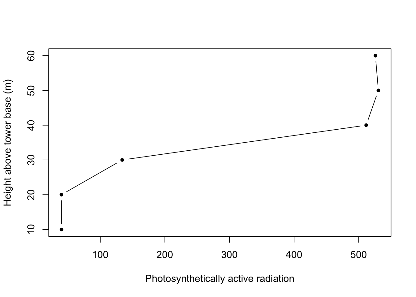
2.11.6.2 Observational data - Terrestrial
Latitude, longitude, elevation, and associated uncertainties are included in
data downloads (Remember NEON COding Lab part 1?). These are the coordinates and uncertainty of the sampling plot;
for many protocols it is possible to calculate a more precise location.
Instructions for doing this are in the respective data product user guides, and
code is in the geoNEON package on GitHub.
2.11.7 Querying a single named location
Let’s look at the named locations in the bird data we downloaded above. To do this,
look for the field called namedLocation, which is present in all observational
data products, both aquatic and terrestrial.
## [1] "WOOD_013.birdGrid.brd" "WOOD_013.birdGrid.brd" "WOOD_013.birdGrid.brd"
## [4] "WOOD_013.birdGrid.brd" "WOOD_013.birdGrid.brd" "WOOD_013.birdGrid.brd"
Here we see the first six entries in the namedLocation column which tells us
the names of the Terrestrial Observation plots where the bird surveys were
conducted.
We can query the locations endpoint of the API for the first named location,
WOOD_013.birdGrid.brd.
# location data
req.loc <- GET("http://data.neonscience.org/api/v0/locations/WOOD_013.birdGrid.brd")

# make this JSON readable
brd.WOOD_013 <- jsonlite::fromJSON(content(req.loc, as="text"))
brd.WOOD_013
## $data
## $data$locationName
## [1] "WOOD_013.birdGrid.brd"
##
## $data$locationDescription
## [1] "Plot \"WOOD_013\" at site \"WOOD\""
##
## $data$locationType
## [1] "OS Plot - brd"
##
## $data$domainCode
## [1] "D09"
##
## $data$siteCode
## [1] "WOOD"
##
## $data$locationDecimalLatitude
## [1] 47.13912
##
## $data$locationDecimalLongitude
## [1] -99.23243
##
## $data$locationElevation
## [1] 579.31
##
## $data$locationUtmEasting
## [1] 482375.7
##
## $data$locationUtmNorthing
## [1] 5220650
##
## $data$locationUtmHemisphere
## [1] "N"
##
## $data$locationUtmZone
## [1] 14
##
## $data$alphaOrientation
## [1] 0
##
## $data$betaOrientation
## [1] 0
##
## $data$gammaOrientation
## [1] 0
##
## $data$xOffset
## [1] 0
##
## $data$yOffset
## [1] 0
##
## $data$zOffset
## [1] 0
##
## $data$offsetLocation
## NULL
##
## $data$locationProperties
## locationPropertyName locationPropertyValue
## 1 Value for Coordinate source GeoXH 6000
## 2 Value for Coordinate uncertainty 0.28
## 3 Value for Country unitedStates
## 4 Value for County Stutsman
## 5 Value for Elevation uncertainty 0.48
## 6 Value for Filtered positions 121
## 7 Value for Geodetic datum WGS84
## 8 Value for Horizontal dilution of precision 1
## 9 Value for Maximum elevation 579.31
## 10 Value for Minimum elevation 569.79
## 11 Value for National Land Cover Database (2001) grasslandHerbaceous
## 12 Value for Plot dimensions 500m x 500m
## 13 Value for Plot ID WOOD_013
## 14 Value for Plot size 250000
## 15 Value for Plot subtype birdGrid
## 16 Value for Plot type distributed
## 17 Value for Positional dilution of precision 2.4
## 18 Value for Reference Point Position B2
## 19 Value for Slope aspect 238.91
## 20 Value for Slope gradient 2.83
## 21 Value for Soil type order Mollisols
## 22 Value for State province ND
## 23 Value for Subtype Specification ninePoints
## 24 Value for UTM Zone 14N
##
## $data$locationParent
## [1] "WOOD"
##
## $data$locationParentUrl
## [1] "https://data.neonscience.org/api/v0/locations/WOOD"
##
## $data$locationChildren
## [1] "WOOD_013.birdGrid.brd.B2" "WOOD_013.birdGrid.brd.A2"
## [3] "WOOD_013.birdGrid.brd.C3" "WOOD_013.birdGrid.brd.A3"
## [5] "WOOD_013.birdGrid.brd.B3" "WOOD_013.birdGrid.brd.C1"
## [7] "WOOD_013.birdGrid.brd.A1" "WOOD_013.birdGrid.brd.B1"
## [9] "WOOD_013.birdGrid.brd.C2"
##
## $data$locationChildrenUrls
## [1] "https://data.neonscience.org/api/v0/locations/WOOD_013.birdGrid.brd.B2"
## [2] "https://data.neonscience.org/api/v0/locations/WOOD_013.birdGrid.brd.A2"
## [3] "https://data.neonscience.org/api/v0/locations/WOOD_013.birdGrid.brd.C3"
## [4] "https://data.neonscience.org/api/v0/locations/WOOD_013.birdGrid.brd.A3"
## [5] "https://data.neonscience.org/api/v0/locations/WOOD_013.birdGrid.brd.B3"
## [6] "https://data.neonscience.org/api/v0/locations/WOOD_013.birdGrid.brd.C1"
## [7] "https://data.neonscience.org/api/v0/locations/WOOD_013.birdGrid.brd.A1"
## [8] "https://data.neonscience.org/api/v0/locations/WOOD_013.birdGrid.brd.B1"
## [9] "https://data.neonscience.org/api/v0/locations/WOOD_013.birdGrid.brd.C2"Note spatial information under $data$[nameOfCoordinate] and under
$data$locationProperties. Also note $data$locationChildren: these are the
finer scale locations that can be used to calculate precise spatial data for
bird observations.
For convenience, we’ll use the geoNEON package to make the calculations.
First we’ll use getLocByName() to get the additional spatial information
available through the API, and look at the spatial resolution available in the
initial download:
# load the geoNEON package
library(geoNEON)

# extract the spatial data
brd.point.loc <- getLocByName(brd.point)
##
|
| | 0%
|
|========== | 14%
|
|==================== | 29%
|
|============================== | 43%
|
|======================================== | 57%
|
|================================================== | 71%
|
|============================================================ | 86%
|
|======================================================================| 100%# plot bird point locations
# note that decimal degrees is also an option in the data
symbols(brd.point.loc$easting, brd.point.loc$northing,
circles=brd.point.loc$coordinateUncertainty,
xlab="Easting", ylab="Northing", tck=0.01, inches=F)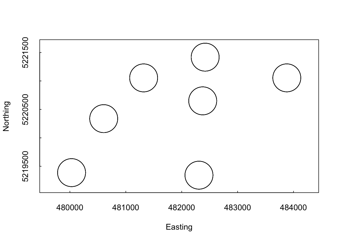
And use getLocTOS() to calculate the point locations of observations.
##
  |
  |                                                                      |   0%
  |
  |=                                                                     |   2%
  |
  |==                                                                    |   3%
  |
  |===                                                                   |   5%
  |
  |====                                                                  |   6%
  |
  |======                                                                |   8%
  |
  |=======                                                               |  10%
  |
  |========                                                              |  11%
  |
  |=========                                                             |  13%
  |
  |==========                                                            |  14%
  |
  |===========                                                           |  16%
  |
  |============                                                          |  17%
  |
  |=============                                                         |  19%
  |
  |==============                                                        |  21%
  |
  |================                                                      |  22%
  |
  |=================                                                     |  24%
  |
  |==================                                                    |  25%
  |
  |===================                                                   |  27%
  |
  |====================                                                  |  29%
  |
  |=====================                                                 |  30%
  |
  |======================                                                |  32%
  |
  |=======================                                               |  33%
  |
  |========================                                              |  35%
  |
  |==========================                                            |  37%
  |
  |===========================                                           |  38%
  |
  |============================                                          |  40%
  |
  |=============================                                         |  41%
  |
  |==============================                                        |  43%
  |
  |===============================                                       |  44%
  |
  |================================                                      |  46%
  |
  |=================================                                     |  48%
  |
  |==================================                                    |  49%
  |
  |====================================                                  |  51%
  |
  |=====================================                                 |  52%
  |
  |======================================                                |  54%
  |
  |=======================================                               |  56%
  |
  |========================================                              |  57%
  |
  |=========================================                             |  59%
  |
  |==========================================                            |  60%
  |
  |===========================================                           |  62%
  |
  |============================================                          |  63%
  |
  |==============================================                        |  65%
  |
  |===============================================                       |  67%
  |
  |================================================                      |  68%
  |
  |=================================================                     |  70%
  |
  |==================================================                    |  71%
  |
  |===================================================                   |  73%
  |
  |====================================================                  |  75%
  |
  |=====================================================                 |  76%
  |
  |======================================================                |  78%
  |
  |========================================================              |  79%
  |
  |=========================================================             |  81%
  |
  |==========================================================            |  83%
  |
  |===========================================================           |  84%
  |
  |============================================================          |  86%
  |
  |=============================================================         |  87%
  |
  |==============================================================        |  89%
  |
  |===============================================================       |  90%
  |
  |================================================================      |  92%
  |
  |==================================================================    |  94%
  |
  |===================================================================   |  95%
  |
  |====================================================================  |  97%
  |
  |===================================================================== |  98%
  |
  |======================================================================| 100%
# plot bird point locations
# note that decimal degrees is also an option in the data
symbols(brd.point.pt$adjEasting, brd.point.pt$adjNorthing,
circles=brd.point.pt$adjCoordinateUncertainty,
xlab="Easting", ylab="Northing", tck=0.01, inches=F)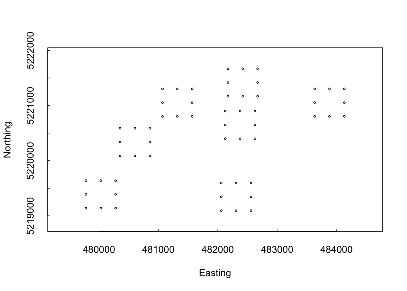
Now you can see the individual points where the respective point counts were located.
2.11.8 Taxonomy
NEON maintains accepted taxonomies for many of the taxonomic identification data we collect. NEON taxonomies are available for query via the API; they are also provided via an interactive user interface, the Taxon Viewer.
NEON taxonomy data provides the reference information for how NEON validates taxa; an identification must appear in the taxonomy lists in order to be accepted into the NEON database. Additions to the lists are reviewed regularly. The taxonomy lists also provide the author of the scientific name, and the reference text used.
The taxonomy endpoint of the API works a little bit differently from the other endpoints. In the “Anatomy of an API Call” section above, each endpoint has a single type of target - a data product number, a named location name, etc. For taxonomic data, there are multiple query options, and some of them can be used in combination. For example, a query for taxa in the Pinaceae family:
http://data.neonscience.org/api/v0/taxonomy/?family=Pinaceae
The available types of queries are listed in the taxonomy section of the API web page. Briefly, they are:
taxonTypeCode: Which of the taxonomies maintained by NEON are you looking for? BIRD, FISH, PLANT, etc. Cannot be used in combination with the taxonomic rank queries.- each of the major taxonomic ranks from genus through kingdom
scientificname: Genus + specific epithet (+ authority). Search is by exact match only, see final example below.verbose: Do you want the short (false) or long (true) responseoffset: Skip this number of items in the list. Defaults to 50.limit: Result set will be truncated at this length. Defaults to 50.
Staff on the NEON project have plans to modify the settings for offset
and limit, such that offset will default to 0 and limit will default
to ∞, but in the meantime users will want to set these manually. They are
set to non-default values in the examples below.
For the first example, let’s query for the loon family, Gaviidae, in the bird taxonomy. Note that query parameters are case-sensitive.
Parse the results into a list using fromJSON():
And look at the $data element of the results, which contains:
- The full taxonomy of each taxon
- The short taxon code used by NEON (taxonID/acceptedTaxonID)
- The author of the scientific name (scientificNameAuthorship)
- The vernacular name, if applicable
- The reference text used (nameAccordingToID)
The terms used for each field are matched to Darwin Core (dwc) and the Global Biodiversity Information Facility (gbif) terms, where possible, and the matches are indicated in the column headers.
##   taxonTypeCode taxonID acceptedTaxonID dwc:scientificName
## 1          BIRD    ARLO            ARLO      Gavia arctica
## 2          BIRD    COLO            COLO        Gavia immer
## 3          BIRD    PALO            PALO     Gavia pacifica
## 4          BIRD    RTLO            RTLO     Gavia stellata
## 5          BIRD    YBLO            YBLO      Gavia adamsii
##   dwc:scientificNameAuthorship dwc:taxonRank dwc:vernacularName
## 1                   (Linnaeus)       species        Arctic Loon
## 2                   (Brunnich)       species        Common Loon
## 3                   (Lawrence)       species       Pacific Loon
## 4                (Pontoppidan)       species  Red-throated Loon
## 5                 (G. R. Gray)       species Yellow-billed Loon
##      dwc:nameAccordingToID dwc:kingdom dwc:phylum dwc:class   dwc:order
## 1 doi: 10.1642/AUK-15-73.1    Animalia   Chordata      Aves Gaviiformes
## 2 doi: 10.1642/AUK-15-73.1    Animalia   Chordata      Aves Gaviiformes
## 3 doi: 10.1642/AUK-15-73.1    Animalia   Chordata      Aves Gaviiformes
## 4 doi: 10.1642/AUK-15-73.1    Animalia   Chordata      Aves Gaviiformes
## 5 doi: 10.1642/AUK-15-73.1    Animalia   Chordata      Aves Gaviiformes
##   dwc:family dwc:genus gbif:subspecies gbif:variety
## 1   Gaviidae     Gavia              NA           NA
## 2   Gaviidae     Gavia              NA           NA
## 3   Gaviidae     Gavia              NA           NA
## 4   Gaviidae     Gavia              NA           NA
## 5   Gaviidae     Gavia              NA           NA
To get the entire list for a particular taxonomic type, use the
taxonTypeCode query. Be cautious with this query, the PLANT taxonomic
list has several hundred thousand entries.
For an example, let’s look up the small mammal taxonomic list, which
is one of the shorter ones, and use the verbose=true option to see
a more extensive list of taxon data, including many taxon ranks that
aren’t populated for these taxa. For space here, we display only
the first 10 taxa:
mam.req <- GET("http://data.neonscience.org/api/v0/taxonomy/?taxonTypeCode=SMALL_MAMMAL&offset=0&limit=500&verbose=true")
mam.list <- jsonlite::fromJSON(content(mam.req, as="text"))
mam.list$data[1:10,]
## taxonTypeCode taxonID acceptedTaxonID dwc:scientificName
## 1 SMALL_MAMMAL AMHA AMHA Ammospermophilus harrisii
## 2 SMALL_MAMMAL AMIN AMIN Ammospermophilus interpres
## 3 SMALL_MAMMAL AMLE AMLE Ammospermophilus leucurus
## 4 SMALL_MAMMAL AMLT AMLT Ammospermophilus leucurus tersus
## 5 SMALL_MAMMAL AMNE AMNE Ammospermophilus nelsoni
## 6 SMALL_MAMMAL AMSP AMSP Ammospermophilus sp.
## 7 SMALL_MAMMAL APRN APRN Aplodontia rufa nigra
## 8 SMALL_MAMMAL APRU APRU Aplodontia rufa
## 9 SMALL_MAMMAL ARAL ARAL Arborimus albipes
## 10 SMALL_MAMMAL ARLO ARLO Arborimus longicaudus
## dwc:scientificNameAuthorship dwc:taxonRank dwc:vernacularName
## 1 Audubon and Bachman species Harriss Antelope Squirrel
## 2 Merriam species Texas Antelope Squirrel
## 3 Merriam species Whitetailed Antelope Squirrel
## 4 Goldman subspecies <NA>
## 5 Merriam species Nelsons Antelope Squirrel
## 6 <NA> genus <NA>
## 7 Taylor subspecies <NA>
## 8 Rafinesque species Sewellel
## 9 Merriam species Whitefooted Vole
## 10 True species Red Tree Vole
## taxonProtocolCategory dwc:nameAccordingToID
## 1 opportunistic isbn: 978 0801882210
## 2 opportunistic isbn: 978 0801882210
## 3 opportunistic isbn: 978 0801882210
## 4 opportunistic isbn: 978 0801882210
## 5 opportunistic isbn: 978 0801882210
## 6 opportunistic isbn: 978 0801882210
## 7 non-target isbn: 978 0801882210
## 8 non-target isbn: 978 0801882210
## 9 target isbn: 978 0801882210
## 10 target isbn: 978 0801882210
## dwc:nameAccordingToTitle
## 1 Wilson D. E. and D. M. Reeder. 2005. Mammal Species of the World; A Taxonomic and Geographic Reference. Third edition. Johns Hopkins University Press; Baltimore, MD.
## 2 Wilson D. E. and D. M. Reeder. 2005. Mammal Species of the World; A Taxonomic and Geographic Reference. Third edition. Johns Hopkins University Press; Baltimore, MD.
## 3 Wilson D. E. and D. M. Reeder. 2005. Mammal Species of the World; A Taxonomic and Geographic Reference. Third edition. Johns Hopkins University Press; Baltimore, MD.
## 4 Wilson D. E. and D. M. Reeder. 2005. Mammal Species of the World; A Taxonomic and Geographic Reference. Third edition. Johns Hopkins University Press; Baltimore, MD.
## 5 Wilson D. E. and D. M. Reeder. 2005. Mammal Species of the World; A Taxonomic and Geographic Reference. Third edition. Johns Hopkins University Press; Baltimore, MD.
## 6 Wilson D. E. and D. M. Reeder. 2005. Mammal Species of the World; A Taxonomic and Geographic Reference. Third edition. Johns Hopkins University Press; Baltimore, MD.
## 7 Wilson D. E. and D. M. Reeder. 2005. Mammal Species of the World; A Taxonomic and Geographic Reference. Third edition. Johns Hopkins University Press; Baltimore, MD.
## 8 Wilson D. E. and D. M. Reeder. 2005. Mammal Species of the World; A Taxonomic and Geographic Reference. Third edition. Johns Hopkins University Press; Baltimore, MD.
## 9 Wilson D. E. and D. M. Reeder. 2005. Mammal Species of the World; A Taxonomic and Geographic Reference. Third edition. Johns Hopkins University Press; Baltimore, MD.
## 10 Wilson D. E. and D. M. Reeder. 2005. Mammal Species of the World; A Taxonomic and Geographic Reference. Third edition. Johns Hopkins University Press; Baltimore, MD.
## dwc:kingdom gbif:subkingdom gbif:infrakingdom gbif:superdivision
## 1 Animalia NA NA NA
## 2 Animalia NA NA NA
## 3 Animalia NA NA NA
## 4 Animalia NA NA NA
## 5 Animalia NA NA NA
## 6 Animalia NA NA NA
## 7 Animalia NA NA NA
## 8 Animalia NA NA NA
## 9 Animalia NA NA NA
## 10 Animalia NA NA NA
## gbif:division gbif:subdivision gbif:infradivision gbif:parvdivision
## 1 NA NA NA NA
## 2 NA NA NA NA
## 3 NA NA NA NA
## 4 NA NA NA NA
## 5 NA NA NA NA
## 6 NA NA NA NA
## 7 NA NA NA NA
## 8 NA NA NA NA
## 9 NA NA NA NA
## 10 NA NA NA NA
## gbif:superphylum dwc:phylum gbif:subphylum gbif:infraphylum gbif:superclass
## 1 NA Chordata NA NA NA
## 2 NA Chordata NA NA NA
## 3 NA Chordata NA NA NA
## 4 NA Chordata NA NA NA
## 5 NA Chordata NA NA NA
## 6 NA Chordata NA NA NA
## 7 NA Chordata NA NA NA
## 8 NA Chordata NA NA NA
## 9 NA Chordata NA NA NA
## 10 NA Chordata NA NA NA
## dwc:class gbif:subclass gbif:infraclass gbif:superorder dwc:order
## 1 Mammalia NA NA NA Rodentia
## 2 Mammalia NA NA NA Rodentia
## 3 Mammalia NA NA NA Rodentia
## 4 Mammalia NA NA NA Rodentia
## 5 Mammalia NA NA NA Rodentia
## 6 Mammalia NA NA NA Rodentia
## 7 Mammalia NA NA NA Rodentia
## 8 Mammalia NA NA NA Rodentia
## 9 Mammalia NA NA NA Rodentia
## 10 Mammalia NA NA NA Rodentia
## gbif:suborder gbif:infraorder gbif:section gbif:subsection gbif:superfamily
## 1 NA NA NA NA NA
## 2 NA NA NA NA NA
## 3 NA NA NA NA NA
## 4 NA NA NA NA NA
## 5 NA NA NA NA NA
## 6 NA NA NA NA NA
## 7 NA NA NA NA NA
## 8 NA NA NA NA NA
## 9 NA NA NA NA NA
## 10 NA NA NA NA NA
## dwc:family gbif:subfamily gbif:tribe gbif:subtribe dwc:genus
## 1 Sciuridae Xerinae Marmotini NA Ammospermophilus
## 2 Sciuridae Xerinae Marmotini NA Ammospermophilus
## 3 Sciuridae Xerinae Marmotini NA Ammospermophilus
## 4 Sciuridae Xerinae Marmotini NA Ammospermophilus
## 5 Sciuridae Xerinae Marmotini NA Ammospermophilus
## 6 Sciuridae Xerinae Marmotini NA Ammospermophilus
## 7 Aplodontiidae <NA> <NA> NA Aplodontia
## 8 Aplodontiidae <NA> <NA> NA Aplodontia
## 9 Cricetidae Arvicolinae <NA> NA Arborimus
## 10 Cricetidae Arvicolinae <NA> NA Arborimus
## dwc:subgenus gbif:subspecies gbif:variety gbif:subvariety gbif:form
## 1 <NA> NA NA NA NA
## 2 <NA> NA NA NA NA
## 3 <NA> NA NA NA NA
## 4 <NA> NA NA NA NA
## 5 <NA> NA NA NA NA
## 6 <NA> NA NA NA NA
## 7 <NA> NA NA NA NA
## 8 <NA> NA NA NA NA
## 9 <NA> NA NA NA NA
## 10 <NA> NA NA NA NA
## gbif:subform speciesGroup dwc:specificEpithet dwc:infraspecificEpithet
## 1 NA <NA> harrisii <NA>
## 2 NA <NA> interpres <NA>
## 3 NA <NA> leucurus <NA>
## 4 NA <NA> leucurus tersus
## 5 NA <NA> nelsoni <NA>
## 6 NA <NA> sp. <NA>
## 7 NA <NA> rufa nigra
## 8 NA <NA> rufa <NA>
## 9 NA <NA> albipes <NA>
## 10 NA <NA> longicaudus <NA>To get information about a single taxon, use the scientificname
query. This query will not do a ‘fuzzy match’, so you need to query
the exact name of the taxon in the NEON taxonomy. Because of this,
the query will be most useful when you already have NEON data in
hand and are looking for more information about a specific taxon.
Querying on scientificname is unlikely to be an efficient way to
figure out if NEON recognizes a particular taxon.
In addition, scientific names contain spaces, which are not allowed in a URL. The spaces need to be replaced with the URL encoding replacement, %20.
For an example, let’s look up the little sand verbena, Abronia
minor Standl. Searching for Abronia minor will fail, because
the NEON taxonomy for this species includes the authority. The
search will also fail with spaces. Search for
Abronia%20minor%20Standl., and in this case we can omit
offset and limit because we know there can only be a single
result:
am.req <- GET("http://data.neonscience.org/api/v0/taxonomy/?scientificname=Abronia%20minor%20Standl.")
am.list <- jsonlite::fromJSON(content(am.req, as="text"))
am.list$data
## taxonTypeCode taxonID acceptedTaxonID dwc:scientificName
## 1 PLANT ABMI2 ABMI2 Abronia minor Standl.
## dwc:scientificNameAuthorship dwc:taxonRank dwc:vernacularName
## 1 Standl. species little sand verbena
## dwc:nameAccordingToID dwc:kingdom dwc:phylum
## 1 http://plants.usda.gov (accessed 8/25/2014) Plantae Magnoliophyta
## dwc:class dwc:order dwc:family dwc:genus gbif:subspecies
## 1 Magnoliopsida Caryophyllales Nyctaginaceae Abronia NA
## gbif:variety
## 1 NA2.12 Stacking NEON data
At the top of this tutorial, we installed the neonUtilities package.
This is a custom R package that stacks the monthly files provided by
the NEON data portal into a single continuous file for each type of
data table in the download. It currently handles files downloaded from
the data portal, but not files pulled from the API.
For a guide to using neonUtilities on data downloaded from the portal,
look here.
2.13 Intro to NEON Exercises: Written Questions
2.14 Intro to NEON Exercises Part 2
2.14.1 Written
Suggested Timing: Complete this exercise before our next class meeting
Question 1: How does NEON address ‘dark data’ (Chapter 1)?
Question 2: How might or does the NEON project intersect with your current research or future career goals? (1 paragraph)Question 3: Use the map in Chapter 2:Intro to NEON to answer the following questions. Consider the research question that you may explore as your final semester project or a current project that you are working on and answer each of the following questions:
- Are there NEON field sites that are in study regions of interest to you?
- What domains are the sites located in?
- What NEON field sites do your current research or Capstone Project ideas
coincide with?
- Is the site or sites core or relocatable?
- Are they terrestrial or aquatic?
- Are there data available for the NEON field site(s) that you are most interested in? What kind of data are available?
Question 4: Consider either your current or future research, or a question you’d like to address durring this course and answer each of the following questions:
- Which types of NEON data may be more useful to address these questions?
- What non-NEON data resources could be combined with NEON data to help address your question?
- What challenges, if any, could you foresee when beginning to work with these data?
Question 5: Use the Data Portal tools to investigate the data availability for the field sites you’ve already identified in the previous sections and answer each of the following questions:
- What types of aquatic or terrestrial data are currently available? Remote sensing data?
- Of these, what type of data are you most interested in working with for your project during this course?
- For what time period does the data cover?
- What format is the downloadable file available in?
- Where is the metadata to support this data?
2.14.2 NEON Coding Lab Part 2
2.15 NEON Coding Lab Part 2
Suggested Timing: Complete this exercise a few days before your NEON clumination write up
- Use the answers that you’ve provided above to select a single NEON site.
e.g. ONAQ
- Use the answers that you’ve provided above to select 3 NEON data products from either the TOS, TIS or ARS (AOP) collection methods. Sumarize each product with its NEON identifier, along with a sumarry.
e.g.:
<<<<<<< HEAD
**DP1.10055.001**: Plant phenology observations: phenophase status and insensity of tagged plants. This data product contains the quality-controlled, native sampling resolution data from in-situ observations of plant leaf development and reproductive phenophases, at **D15.ONAQ**.
Using the NEON Ulitites package or the API pull in those data along with metadata.
Organize your data into
data.framesand produce summaries for each of your data:Filter your data based on metadata and quality flags:
DP1.10055.001: Plant phenology observations: phenophase status and intensity of tagged plants. This data product contains the quality-controlled, native sampling resolution data from in-situ observations of plant leaf development and reproductive phenophases, at D15.ONAQ. Here I will focus on the phenophase intensity data, which is a measure of how prevalent that particular phenophase is in the sampled plants.
- Using the NEON Ulitites package or the API pull in those data along with metadata.
sitesOfInterest <- c("ONAQ")

dpid <- as.character('DP1.10055.001') #phe data

pheDat <- loadByProduct(dpID="DP1.10055.001",
                     site = sitesOfInterest,
                     package = "basic",
                     check.size = FALSE,
token=NEON_TOKEN)- Organize your data into
data.framesand produce summaries for each of your data:
#NEON sends the data as a nested list, so I need to undo that
# unlist all data frames
list2env(pheDat ,.GlobalEnv)
summary(phe_perindividualperyear)
summary(phe_statusintensity)- Filter and format your data based on metadata and quality flags:
#remove duplicate records
phe_statusintensity <- select(phe_statusintensity, -uid)
phe_statusintensity <- distinct(phe_statusintensity)
#Format dates (native format is 'factor' silly R)
phe_statusintensity$date <- as.Date(phe_statusintensity$date, "%Y-%m-%d")
phe_statusintensity$editedDate <- as.Date(phe_statusintensity$editedDate, "%Y-%m-%d")
phe_statusintensity$year <- substr(phe_statusintensity$date, 1, 4)
phe_statusintensity$monthDay <- format(phe_statusintensity$date, format="%m-%d")
Now I want to remove NA values so I can see what’s really going on:
- Create minimum of 1 plot per data type (minimum of 3 plots total). These will vary based on that data that you’ve chosen.
A non-exhastive list of ideas: 1. Your data as a function of height on the tower (FPAR example) 2. A map of the locations where your data is sampled (TOS tree example, bird example) 3. A model based on the data you’re interested in working work (Coding lab 1 example) 4. A timeseries of your data (example below)
- What is the frequency of the data you decided was of interest? How do the data align to answer a central question? What challenges did you run into when investigating these data? How will you address these challenges and document your code? One to two paragraphs
Intro to NEON Culmination Activity
- What is the temporal frequency of observations in the data you decided was of interest? How do the data align to answer a central question? What challenges did you run into when investigating these data? How will you address these challenges and document your code? One to two paragraphs
2.16 Intro to NEON Culmination Activity
Due before we start Chapter 3: USA-NPN >>>>>>> upstream/master
Write up a 1-page summary of a project that you might want to explore using NEON data over the duration of this course. Include:
- the types of NEON (and other data) that you will need to implement this project, including data product id numbers.
- If in your NEON coding lab part 2 you highlighted challenges to using these data, discuss methods to address those challenges. *e.g. If your site doesn’t yet have a long data recocrd, is it located close to a longer lived site from another network? (LTER, Ameriflux, LTAR etc)
- One high-level summary graphic including all of your data from the NEON Coding Lab Part 2
Save this summary as you will be refining and adding to your ideas over the course of the semester.