Chapter 8 USGS National Water Information System (NWIS)
United States Geological Survey’s National Water Information System (NWIS)
8.1 USGS Mission:
Changes to the natural world combined with growing human demands put our health and safety, national security, and economy at risk. We are focused on some of the most significant issues society faces, and our science is making a substantial contribution to the well-being of the Nation and the world.
You can explore USGS Missions and programs here.
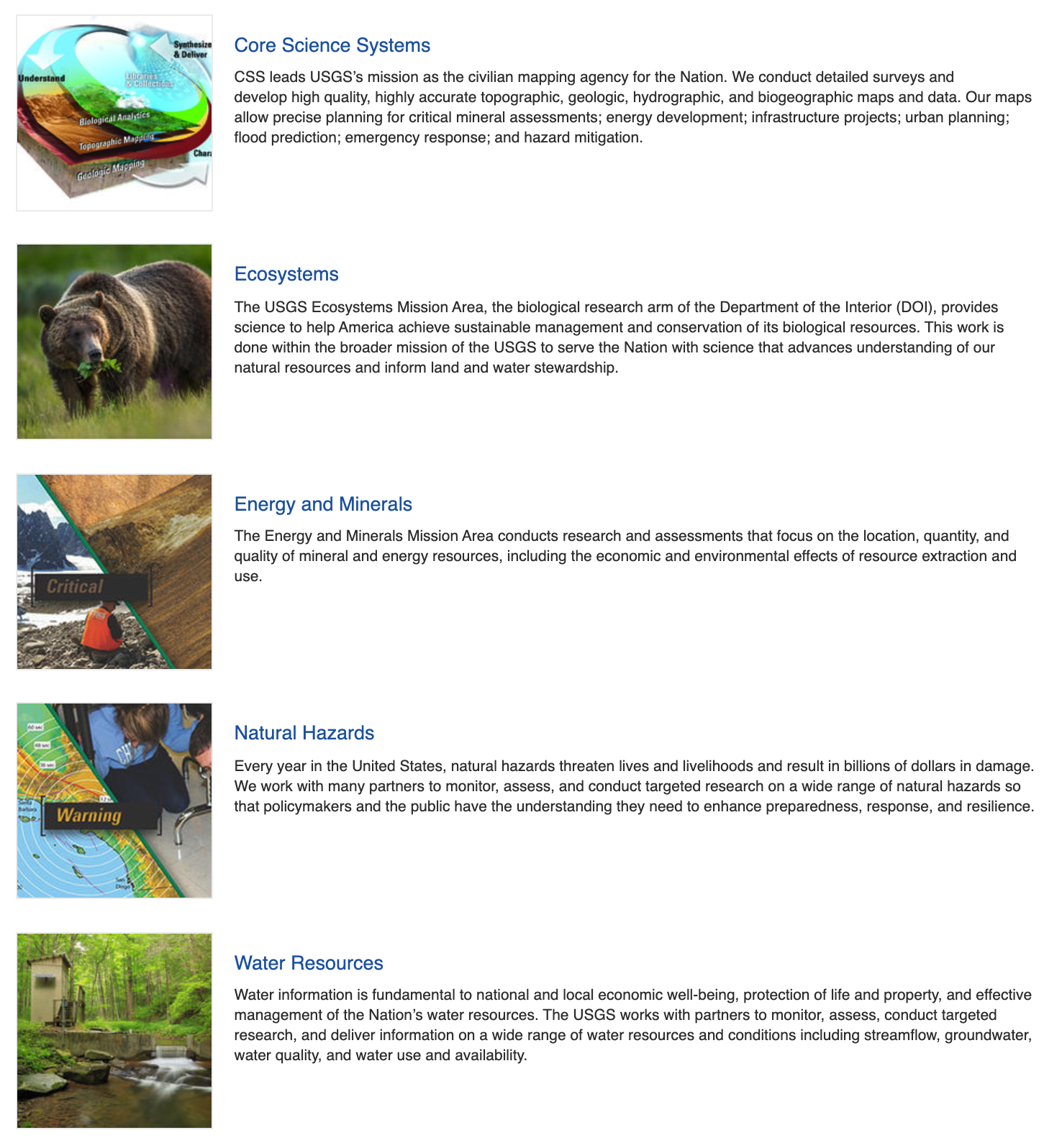
8.2 USGS Water Resources Mission:
Water information is fundamental to national and local economic well-being, protection of life and property, and effective management of the Nation’s water resources. The USGS works with partners to monitor, assess, conduct targeted research, and deliver information on a wide range of water resources and conditions including streamflow, groundwater, water quality, and water use and availability.
The United States Geological Survey (USGS) has collected water-resources data at approximately 1.5 million sites in all 50 States, the District of Columbia, Puerto Rico, the Virgin Islands, Guam, American Samoa and the Commonwealth of the Northern Mariana Islands.
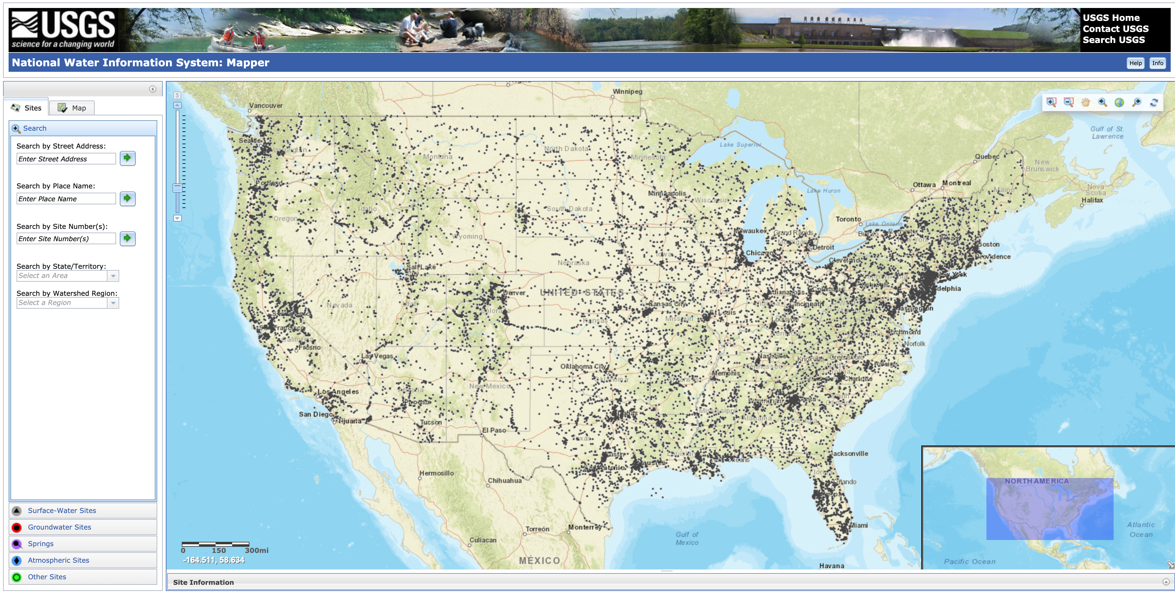
A map of collection sites can be found here
8.3 Types of USGS NWIS Data
The types of data collected are varied, but generally fit into the broad categories of surface water and groundwater.
Surface-water data, such as gage height (stage) and streamflow (discharge), are collected at major rivers, lakes, and reservoirs.
Groundwater data, such as water level, are collected at wells and springs.
Water-quality data are available for both surface water and groundwater. Examples of water-quality data collected are temperature, specific conductance, pH, nutrients, pesticides, and volatile organic compounds.
The NWIS web site serves current and historical data. Data are retrieved by category of data, such as surface water, groundwater, or water quality, and by geographic area.
8.4 USGS R Packages: Collaborative and reproducible data analysis using R
Contributors: Jordan Read, Lindsay Carr Adapted from USGS ‘Getting Started with USGS R Packages’ course materials
Recently, the USGS has built a suite of software packages and tutorials for R users to to interact with their data and streamline workflows. Here we have adapted course materials from thier USGS R packages course materials written and developed by Lindsay R. Carr.
The common workflow for completing the data processing pipeline is subject to human error at every step: accessing data, analyzing data, and producing final figures. Multi-site analyses are especially error-prone because the same workflow needs to be repeated many times. This course teaches a modular approach to the common data analysis workflow by building on basic R data analysis skills and leveraging existing USGS R packages that can create advanced, reproducible workflows, such as for accessing gridded climate data, analyzing high frequency water observations, and for taking full advantage of the USGS ScienceBase repository. The USGS packages covered in this course span a variety of applications: accessing web data, accessing personally stored data, and releasing data for publication.
The modular workflows taught in this section will prepare researchers to create automated, robust data processing workflows through more efficient code development. Following the course, students will be capable of integrating these packages into their own scientific workflows.
8.4.1 Suggested prerequisite knowledge
This course assumes a moderate to advanced knowledge of the statistical programming language R. If you’re interested in using USGS packages for data analysis but have no R experience, please visit the Introduction to R curriculum available at this site.
- Experience using R to import, view, and summarize data
- Recommended: experience creating simple plots in R
- Recommended: familiarity with RStudio
8.4.2 Course outline
## Warning: package 'htmlTable' was built under R version 3.6.2|
|
||
| Module | Description | Duration |
|---|---|---|
| dataRetrieval | Accessing time series data. | 2 hours |
| geoknife | Accessing gridded data. | 1 hour |
| Application | Use the packages introduced in previous modules to create and use a robust modular workflow. | 1.5 hour |
8.4.3 Software requirements
See the R installation instructions page for how to install/upgrade R and RStudio, add GRAN to your settings, and install some basic packages. Then, execute these lines so that you have the most up-to-date version of the packages used in this course.
8.4.4 Lesson Summary
This lesson will focus on finding and retrieving hydrologic time series data using the USGS R package, dataRetrieval. The package was created to make querying and downloading hydrologic data from the web easier, less error-prone, and reproducible. The package allows users to easily access data stored in the USGS National Water Information System (NWIS) and the multi-agency database, Water Quality Portal (WQP). NWIS only contains data collected by or for the USGS. Conversely, WQP is a database that aggregates water quality data from multiple agencies, including USGS, Environmental Protection Agency (EPA), US Department of Agriculture (USDA), and many state, tribal, and local agencies.
dataRetrieval functions take user-defined arguments and construct web service calls. The web service returns the data as XML (a standard data structure), and dataRetrieval takes care of parsing that into a useable R data.frame, complete with metadata. When web services change, dataRetrieval users aren’t affected because the package maintainers will update the functions to handle these modifications. This is what makes dataRetrieval so user-friendly.
Neither NWIS nor WQP are static databases. Users should be aware that data is constantly being added, so a query one week might return differing amounts of data from the next. For more information about NWIS, please visit waterdata.usgs.gov/nwis. For more information about WQP, visit their site www.waterqualitydata.us or read about WQP for aquatic research applications in the publication, Water quality data for national-scale aquatic research: The Water Quality Portal.
8.4.5 Lesson Objectives
Learn about data available in the National Water Information System (NWIS) and Water Quality Portal (WQP). Discover how to construct your retrieval calls to get exactly what you are looking for, and access information stored as metadata in the R object.
By the end of this lesson, the learner will be able to:
- Investigate what data are available in National Water Information System (NWIS) and Water Quality Portal (WQP) through package functions.
- Construct function calls to pull a variety of NWIS and WQP data.
- Access metadata information from retrieval call output.
8.4.6 Lesson Resources
- USGS publication: The dataRetrieval R package
- Source code: dataRetrieval on GitHub
- Report a bug or suggest a feature: dataRetrieval issues on GitHub
- USGS Presentation: dataRetrieval Tutorial
8.4.7 Lesson Slide Deck
Browse the slide deck here
8.5 Introduction to USGS R Packages
Before continuing with this lesson, you should make sure that the dataRetrieval package is installed and loaded. If you haven’t recently updated, you could reinstall the package by running install.packages('dataRetrieval') or go to the “Update” button in the “Packages” tab in RStudio.
There is an overwhelming amount of data and information stored in the National Water Information System (NWIS). This lesson will attempt to give an overview of what you can access. If you need more detail on a subject or have a question that is not answered here, please visit the NWIS help system.
8.6 Data available
Data types: NWIS and WQP store a lot of water information. NWIS contains streamflow, peak flow, rating curves, groundwater, and water quality data. As can be assumed from the name, WQP only contains water quality data.
Time series types: the databases store water data at various reporting frequencies, and have different language to describe these. There are 3 main types: unit value, daily value, and discrete. WQP only contains discrete data.
- instantaneous value (sometimes called unit value) data is reported at the frequency in which it was collected, and includes real-time data. It is generally available from 2007-present.
- daily value data aggregated to a daily statistic (e.g. mean daily, minimum daily, or maximum daily). This is available for streamflow, groundwater levels, and water quality sensors.
- discrete data collected at a specific point in time, and is not a continuous time series. This includes most water quality data, groundwater levels, rating curves, surface water measurements, and peak flow.
Metadata types: both NWIS and WQP contain metadata describing the site at which the data was collected (e.g. latitude, longitude, elevation, etc), and include information about the type of data being used (e.g. units, dissolved or not, collection method, etc).
8.7 Common NWIS function arguments
siteNumber All NWIS data are stored based on the geographic location of the equipment used to collected the data. These are known as streamgages and they take continuous timeseries measurements for a number of water quality and quantity parameters. Streamgages are identified based on an 8-digit (surface water) or 15-digit (groundwater) code. In dataRetrieval, we refer to this as the siteNumber. Any time you use a siteNumber in dataRetrieval, make sure it is a string and not numeric. Oftentimes, NWIS sites have leading zeroes which are dropped when treated as a numeric value.
parameterCd NWIS uses 5-digit codes to refer to specific data of interest called parameter codes, parameterCd in dataRetrieval. For example, you use the code ‘00060’ to specify discharge data. If you’d like to explore the full list, see the Parameter Groups Table. The package also has a built in parameter code table that you can use by executing parameterCdFile in your console.
service Identifier referring to the time series frequencies explained above, or the type of data that should be returned. For more information, visit the Water Services website.
- instaneous = “iv”
- daily values = “dv”
- groundwater levels = “gwlevels”
- water quality = “qw”
- statistics = “stat”
- site = “site”
startDate and endDate Strings in the format “YYYY-MM-DDTHH:SS:MM”, either as a date or character class. The start and end date-times are inclusive.
stateCd Two character abbreviation for a US state or territory. Execute state.abb in the console to get a vector of US state abbreviations. Territories include:
- AS (American Samoa)
- GU (Guam)
- MP (Northern Mariana Islands)
- PR (Puerto Rico)
- VI (U.S. Virgin Islands)
For more query parameters, visit NWIS service documentation.
8.8 Discovering NWIS data
In some cases, users might have specific sites and data that they are pulling with dataRetrieval but what if you wanted to know what data exists in the database before trying to download it? You can use the function whatNWISdata, described below. Another option is to download the data using readNWISdata, and see the first and last available dates of that data with the arguments seriesCatalogOutput=TRUE and service="site". Downloading data will be covered in the next section, readNWIS.
8.8.1 whatNWISdata
whatNWISdata will return a data.frame specifying the types of data available for a specified major filter that fits your querying criteria. You can add queries by the data service, USGS parameter code, or statistics code. You need at least one “major filter” in order for the query to work. “Major filters” include siteNumber, stateCd, huc, bBox, or countyCd.
In this example, let’s find South Carolina stream temperature data. We specify the state, South Carolina, using the stateCd argument and South Carolina’s two letter abbreviation, SC.
## [1] 186041Let’s look at the dataframe returned from whatNWISdata:
##   agency_cd  site_no                station_nm site_tp_cd dec_lat_va
## 1      USGS 02110400 BUCK CREEK NEAR LONGS, SC         ST    33.9535
## 2      USGS 02110400 BUCK CREEK NEAR LONGS, SC         ST    33.9535
## 3      USGS 02110400 BUCK CREEK NEAR LONGS, SC         ST    33.9535
## 4      USGS 02110400 BUCK CREEK NEAR LONGS, SC         ST    33.9535
## 5      USGS 02110400 BUCK CREEK NEAR LONGS, SC         ST    33.9535
## 6      USGS 02110400 BUCK CREEK NEAR LONGS, SC         ST    33.9535
##   dec_long_va coord_acy_cd dec_coord_datum_cd alt_va alt_acy_va alt_datum_cd
## 1   -78.71974            S              NAD83   5.30        .01       NAVD88
## 2   -78.71974            S              NAD83   5.30        .01       NAVD88
## 3   -78.71974            S              NAD83   5.30        .01       NAVD88
## 4   -78.71974            S              NAD83   5.30        .01       NAVD88
## 5   -78.71974            S              NAD83   5.30        .01       NAVD88
## 6   -78.71974            S              NAD83   5.30        .01       NAVD88
##     huc_cd data_type_cd parm_cd stat_cd  ts_id loc_web_ds medium_grp_cd
## 1 03040206           ad    <NA>    <NA>      0       <NA>           wat
## 2 03040206           dv   00010   00001 124327       <NA>           wat
## 3 03040206           dv   00010   00002 124328       <NA>           wat
## 4 03040206           dv   00010   00003 124329       <NA>           wat
## 5 03040206           dv   00045   00006 124351       <NA>           wat
## 6 03040206           dv   00060   00001 124348       <NA>           wat
##   parm_grp_cd  srs_id access_cd begin_date   end_date count_nu
## 1        <NA>       0         0 2006-01-01 2019-01-01       14
## 2        <NA> 1645597         0 2005-10-01 2020-10-12     5395
## 3        <NA> 1645597         0 2005-10-01 2020-10-12     5395
## 4        <NA> 1645597         0 2005-10-01 2020-10-12     5395
## 5        <NA> 1644459         0 2006-01-06 2020-10-12     5203
## 6        <NA> 1645423         0 2005-11-17 2019-08-17     4394
The data returned from this query can give you information about the data available for each site including, date of first and last record (begin_date, end_date), number of records (count_nu), site altitude (alt_va), corresponding hydrologic unit code (huc_cd), and parameter units (parameter_units). These columns allow even more specification of data requirements before actually downloading the data. This function returns one row per unique combination of site number, dates, parameter, etc. In order to just get the sites, use unique:
## [1] 10127To be more specific, let’s say we only want stream sites. This requires the siteType argument and the abbreviation “ST” for stream. See other siteTypes here. We also only want to use sites that have temperature data (USGS parameter code is 00010). Use the argument parameterCd and enter the code as a character string, otherwise leading zeroes will be dropped. Recall that you can see a table of all parameter codes by executing parameterCdFile in your console.
data_sc_stream_temp <- whatNWISdata(stateCd="SC", siteType="ST", parameterCd="00010")
nrow(data_sc_stream_temp)
## [1] 652We are now down to just 652 rows of data, much less than our original 186,041 rows. Downloading NWIS data will be covered in the next section, readNWIS.
The whatNWISdata function can also be very useful for making quick maps with site locations, see the columns dec_lat_va and dec_long_va (decimal latitude and longitude value). For instance,
# SC stream temperature sites
library(maps)
map('state', regions='south carolina')
title(main="South Carolina Stream Temp Sites")
points(x=data_sc_stream_temp$dec_long_va,
       y=data_sc_stream_temp$dec_lat_va)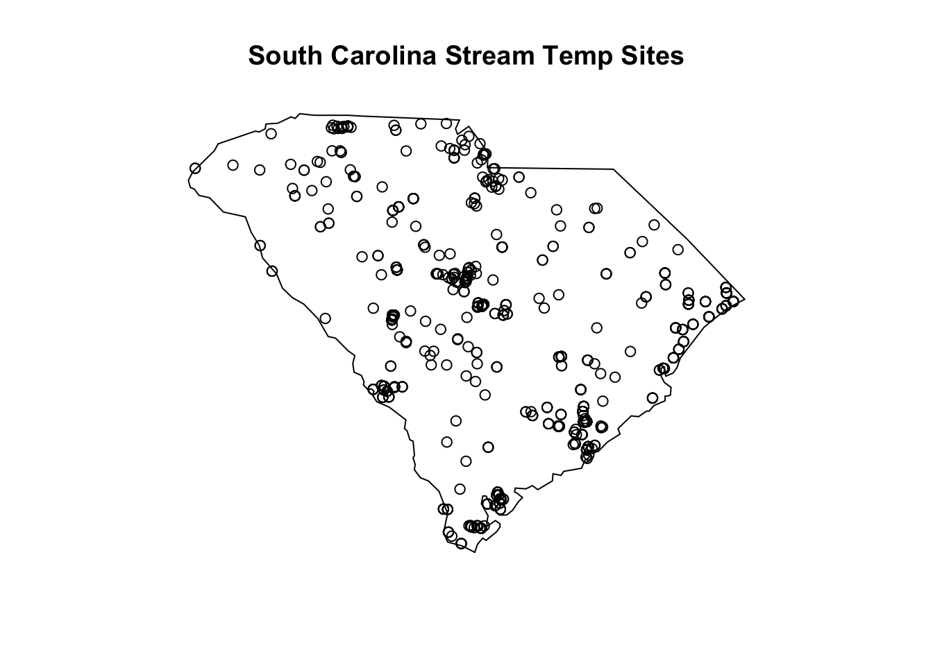
(#fig:sc_streamtemp_data_map)Geographic locations of NWIS South Carolina stream sites with temperature data
Continuing with the South Carolina temperature data example, let’s look for the mean daily stream temperature.
# Average daily SC stream temperature data
data_sc_stream_temp_avg <- whatNWISdata(
  stateCd="SC",
  siteType="ST",
  parameterCd="00010",
  service="dv",
  statCd="00003")
nrow(data_sc_stream_temp_avg)
## [1] 95Let’s apply an additional filter to these data using the filter function from dplyr. Imagine that the trend analysis you are conducting requires a minimum of 300 records and the most recent data needs to be no earlier than 1975.
# Useable average daily SC stream temperature data
library(dplyr)
data_sc_stream_temp_avg_applicable <- data_sc_stream_temp_avg %>%
  filter(count_nu >= 300, end_date >= "1975-01-01")
nrow(data_sc_stream_temp_avg_applicable)
## [1] 91This means you would have 91 sites to work with for your study.
8.9 Common WQP function arguments
countrycode, statecode, and countycode These geopolitical filters can be specified by a two letter abbreviation, state name, or Federal Information Processing Standard (FIPS) code. If you are using the FIPS code for a state or county, it must be preceded by the FIPS code of the larger geopolitical filter. For example, the FIPS code for the United States is US, and the FIPS code for South Carolina is 45. When querying with the statecode, you can enter statecode="US:45". The same rule extends to county FIPS; for example, you can use countycode="45:001" to query Abbeville County, South Carolina. You can find all state and county codes and abbreviations by executing stateCd or countyCd in your console.
siteType Specify the hydrologic location the sample was taken, e.g. streams, lakes, groundwater sources. These should be listed as a string. Available types can be found here.
organization The ID of the reporting organization. All USGS science centers are written “USGS-” and then the two-letter state abbrevation. For example, the Wisconsin Water Science Center would be written “USGS-WI”. For all available organization IDs, please see this list of org ids. The id is listed in the “value” field, but they are accompanied by the organization name in the “desc” (description) field.
siteid This is the unique identification number associated with a data collection station. Site IDs for the same location may differ depending on the reporting organization. The site ID string is written as the agency code then the site number separated by a hyphen. For example, the USGS site 01594440 would be written as “USGS-01594440”.
characteristicName and characteristicType Unlike NWIS, WQP does not have codes for each parameter. Instead, you need to search based on the name of the water quality constituent (referred to as characteristicName in dataRetrieval) or a group of parameters (characteristicType in dataRetrieval). For example, “Nitrate” is a characteristicName and “Nutrient” is the characteristicType that it fits into. For a complete list of water quality types and names, see characteristicType list and characteristicName list.
startDate and endDate Arguments specifying the beginning and ending of the period of record you are interested in. For the dataRetrieval functions, these can be a date or character class in the form YYYY-MM-DD. For example, startDate = as.Date("2010-01-01") or startDate = "2010-01-01" could both be your input arguments.
8.10 Discovering WQP data
WQP has millions of records, and if you aren’t careful, your query could take hours because of the amount of data that met your criteria. To avoid this, you can query just for the number of records and number of sites that meet your criteria using the argument querySummary=TRUE in the function, readWQPdata. See the lesson on downloading WQP data to learn more about getting data. You can also use whatWQPsites to get the site information that matches your criteria.
Let’s follow a similar pattern to NWIS data discovery sections and explore available stream temperature data in South Carolina.
8.10.1 readWQPdata + querySummary
readWQPdata is the function used to actually download WQP data. In this application, we are just querying for a count of sites and results that match our criteria. Since WQP expect state and county codes as their FIPS code, you will need to use the string “US:45” for South Carolina.
##  [1] "content-type"              "content-length"
##  [3] "server"                    "date"
##  [5] "content-disposition"       "total-site-count"
##  [7] "nwis-site-count"           "storet-site-count"
##  [9] "total-activity-count"      "nwis-activity-count"
## [11] "storet-activity-count"     "total-result-count"
## [13] "nwis-result-count"         "storet-result-count"
## [15] "x-frame-options"           "x-content-type-options"
## [17] "x-xss-protection"          "strict-transport-security"
## [19] "x-cache"                   "via"
## [21] "x-amz-cf-pop"              "x-amz-cf-id"
This returns a list with 22 different items, including total number of sites, breakdown of the number of sites by source (BioData, NWIS, STORET), total number of records, and breakdown of records count by source. Let’s just look at total number of sites and total number of records.
## [1] 7101## [1] 3647355This doesn’t provide any information about the sites, just the total number. I know that with 3,647,355 results, I will want to add more criteria before trying to download. Let’s continue to add query parameters before moving to whatWQPsites.
# specify that you only want data from streams
wqpcounts_sc_stream <- readWQPdata(statecode="US:45", siteType="Stream",
                                  querySummary = TRUE)
wqpcounts_sc_stream[['total-site-count']]
## [1] 2006## [1] 18619231,861,923 results are still a lot to download. Let’s add more levels of criteria:
# specify that you want water temperature data and it should be from 1975 or later
wqpcounts_sc_stream_temp <- readWQPdata(statecode="US:45", siteType="Stream",
                                       characteristicName="Temperature, water",
                                       startDate="1975-01-01",
                                       querySummary = TRUE)
wqpcounts_sc_stream_temp[['total-site-count']]
## [1] 1467## [1] 141508141,508 is little more manageble. We can also easily compare avilable stream temperature and lake temperature data.
wqpcounts_sc_lake_temp <- readWQPdata(statecode="US:45",
                                      siteType="Lake, Reservoir, Impoundment",
                                      characteristicName="Temperature, water",
                                      startDate="1975-01-01",
                                      querySummary = TRUE)
# comparing site counts
wqpcounts_sc_stream_temp[['total-site-count']]
## [1] 1467## [1] 636## [1] 141508## [1] 52700From these query results, it looks like South Carolina has much more stream data than it does lake data.
Now, let’s try our South Carolina stream temperature query with whatWQPsites and see if we can narrow the results at all.
8.10.2 whatWQPsites
whatWQPsites gives back site information that matches your search criteria. You can use any of the regular WQP web service arguments here. We are going to use whatWQPsites with the final criteria of the last query summary call - state, site type, parameter, and the earliest start date. This should return the same amount of sites as the last readWQPdata query did, 1,467.
# Getting the number of sites and results for stream
# temperature measurements in South Carolina after 1975.
wqpsites_sc_stream_temp <- whatWQPsites(statecode="US:45", siteType="Stream",
                                       characteristicName="Temperature, water",
                                       startDate="1975-01-01")
# number of sites
nrow(wqpsites_sc_stream_temp)
## [1] 1467## [1] "OrganizationIdentifier"
## [2] "OrganizationFormalName"
## [3] "MonitoringLocationIdentifier"
## [4] "MonitoringLocationName"
## [5] "MonitoringLocationTypeName"
## [6] "MonitoringLocationDescriptionText"
## [7] "HUCEightDigitCode"
## [8] "DrainageAreaMeasure.MeasureValue"
## [9] "DrainageAreaMeasure.MeasureUnitCode"
## [10] "ContributingDrainageAreaMeasure.MeasureValue"
## [11] "ContributingDrainageAreaMeasure.MeasureUnitCode"
## [12] "LatitudeMeasure"
## [13] "LongitudeMeasure"
## [14] "SourceMapScaleNumeric"
## [15] "HorizontalAccuracyMeasure.MeasureValue"
## [16] "HorizontalAccuracyMeasure.MeasureUnitCode"
## [17] "HorizontalCollectionMethodName"
## [18] "HorizontalCoordinateReferenceSystemDatumName"
## [19] "VerticalMeasure.MeasureValue"
## [20] "VerticalMeasure.MeasureUnitCode"
## [21] "VerticalAccuracyMeasure.MeasureValue"
## [22] "VerticalAccuracyMeasure.MeasureUnitCode"
## [23] "VerticalCollectionMethodName"
## [24] "VerticalCoordinateReferenceSystemDatumName"
## [25] "CountryCode"
## [26] "StateCode"
## [27] "CountyCode"
## [28] "AquiferName"
## [29] "FormationTypeText"
## [30] "AquiferTypeName"
## [31] "ConstructionDateText"
## [32] "WellDepthMeasure.MeasureValue"
## [33] "WellDepthMeasure.MeasureUnitCode"
## [34] "WellHoleDepthMeasure.MeasureValue"
## [35] "WellHoleDepthMeasure.MeasureUnitCode"
## [36] "ProviderName"Similar to what we did with the NWIS functions, we can filter the sites further using the available metadata in wqpsites_sc_stream_temp. We are going to imagine that for our study the sites must have an associated drainage area and cannot be below sea level. Using dplyr::filter:
# Filtering the number of sites and results for stream temperature
# measurements in South Carolina after 1975 to also have an
# associated drainage area and collected above sea level.
wqpsites_sc_stream_temp_applicable <- wqpsites_sc_stream_temp %>%
  filter(!is.na(DrainageAreaMeasure.MeasureValue),
         VerticalMeasure.MeasureValue > 0)

nrow(wqpsites_sc_stream_temp_applicable)
## [1] 74This brings the count down to a much more manageable 74 sites. Now we are ready to download this data.
8.11 readNWIS functions
We have learned how to discover data available in NWIS, but now we will look at how to retrieve data. There are many functions to do this, see the table below for a description of each. Each variation of readNWIS is accessing a different web service. For a definition and more information on each of these services, please see https://waterservices.usgs.gov/rest/. Also, refer to the previous lesson for a description of the major arguments to readNWIS functions.
|
|
||
| Function | Description | Arguments |
|---|---|---|
| readNWISdata | Most general NWIS data import function. User must explicitly define the service parameter. More flexible than the other functions. | …, asDateTime, convertType, tz |
| readNWISdv | Returns time-series data summarized to a day. Default is mean daily. | siteNumbers, parameterCd, startDate, endDate, statCd |
| readNWISgwl | Groundwater levels. | siteNumbers, startDate, endDate, convertType, tz |
| readNWISmeas | Surface water measurements. | siteNumbers, startDate, endDate, tz, expanded, convertType |
| readNWISpCode | Metadata information for one or many parameter codes. | parameterCd |
| readNWISpeak | Annual maximum instantaneous streamflows and gage heights. | siteNumbers, startDate, endDate, asDateTime, convertType |
| readNWISqw | Discrete water quality data. | siteNumbers, parameterCd, startDate, endDate, expanded, reshape, tz |
| readNWISrating | Rating table information for active stream gages | siteNumber, type, convertType |
| readNWISsite | Site metadata information | siteNumbers |
| readNWISstat | Daily, monthly, or annual statistics for time-series data. Default is mean daily. | siteNumbers, parameterCd, startDate, endDate, convertType, statReportType, statType |
| readNWISuse | Data from the USGS National Water Use Program. | stateCd, countyCd, years, categories, convertType, transform |
| readNWISuv | Returns time-series data reported from the USGS Instantaneous Values Web Service. | siteNumbers, parameterCd, startDate, endDate, tz |
Each service-specific function is a wrapper for the more flexible readNWISdata. They set a default for the service argument and have limited user defined arguments. All readNWIS functions require a “major filter” as an argument, but readNWISdata can accept any major filter while others are limited to site numbers or state/county codes (see Table 1 for more info).
Other major filters that can be used in readNWISdata include hydrologic unit codes (huc) and bounding boxes (bBox). More information about major filters can be found in the NWIS web services documentation.
The following are examples of how to use each of the readNWIS family of functions. Don’t forget to load the dataRetrieval library if you are in a new session.
- readNWISdata, county major filter
- readNWISdata, huc major filter
- readNWISdata, bbox major filter
- readNWISdv
- readNWISgwl
- readNWISmeas
- readNWISpCode
- readNWISpeak
- readNWISqw, multiple sites
- readNWISqw, multiple parameters
- readNWISrating, using base table
- readNWISrating, corrected table
- readNWISrating, shift table
- readNWISsite
- readNWISstat
- readNWISuse
- readNWISuv
8.11.1 readNWISdata
This function is the generic, catch-all for pulling down NWIS data. It can accept a number of arguments, but the argument name must be included. To use this function, you need to specify at list one major filter (state, county, site number, huc, or bounding box) and the NWIS service (daily value, instantaneous, groundwater, etc). The rest are optional query parameters. Follow along with the three examples below or see ?readNWISdata for more information.
Historic mean daily streamflow for sites in Maui County, Hawaii.
# Major filter: Maui County
## need to also include the state when using counties as the major filter
# Service: daily value, dv
# Parameter code: streamflow in cfs, 00060

MauiCo_avgdailyQ <- readNWISdata(stateCd="Hawaii", countyCd="Maui", service="dv", parameterCd="00060")
head(MauiCo_avgdailyQ)
## agency_cd site_no dateTime X_00060_00003 X_00060_00003_cd tz_cd
## 1 USGS 16400000 2021-02-11 7.93 P UTC
## 2 USGS 16401000 1929-08-31 18.00 A UTC
## 3 USGS 16402000 1957-07-31 51.00 A UTC
## 4 USGS 16403000 1957-06-30 5.50 A UTC
## 5 USGS 16403600 1970-09-29 2.40 A UTC
## 6 USGS 16403900 1996-09-30 1.30 A UTC## [1] 132Historic minimum water temperatures for the HUC8 corresponding to the island of Maui, Hawaii.
To see all HUCs available, visit https://water.usgs.gov/GIS/huc_name.html. The default statistic for daily values in readNWISdata is to return the max (00001), min (00002), and mean (00003). We will specify the minimum only for this example. You will need to use the statistic code, not the name. For all the available statistic codes, see the statType web service documentation and NWIS table mapping statistic names to codes. Caution! In readNWISdata and readNWISdv the argument is called statCd, but in readNWISstat the argument is statType.
# Major filter: HUC 8 for Maui, 20020000
# Service: daily value, dv
# Statistic: minimum, 00002
# Parameter code: water temperature in deg C, 00010

MauiHUC8_mindailyT <- readNWISdata(huc="20020000", service="dv", statCd="00002", parameterCd="00010")
head(MauiHUC8_mindailyT)
## agency_cd site_no dateTime X_00010_00002 X_00010_00002_cd tz_cd
## 1 USGS 16508000 2003-11-24 17.4 A UTC
## 2 USGS 16516000 2003-11-24 16.3 A UTC
## 3 USGS 16520000 2004-04-14 17.5 A UTC
## 4 USGS 16527000 2004-01-13 15.4 A UTC
## 5 USGS 16555000 2004-01-13 16.4 A UTC
## 6 USGS 16618000 2021-02-11 18.1 P UTC## [1] 47Total nitrogen in mg/L for last 30 days around Great Salt Lake in Utah.
This example uses Sys.Date to get the most recent date, so your dates will differ. To get any data around Great Salt Lake, we will use a bounding box as the major filter. The bounding box must be a vector of decimal numbers indicating the western longitude, southern latitude, eastern longitude, and northern latitude. The vector must be in that order.
# Major filter: bounding box around Great Salt Lake
# Service: water quality, qw
# Parameter code: total nitrogen in mg/L, 00600
# Beginning: this past 30 days, use Sys.Date()

prev30days <- Sys.Date() - 30
SaltLake_totalN <- readNWISdata(bBox=c(-113.0428, 40.6474, -112.0265, 41.7018), service="qw",
                           parameterCd="00600", startDate=prev30days)
# This service returns a lot of columns:
names(SaltLake_totalN)
## [1] "agency_cd" "site_no"
## [3] "sample_dt" "sample_tm"
## [5] "sample_end_dt" "sample_end_tm"
## [7] "sample_start_time_datum_cd" "tm_datum_rlbty_cd"
## [9] "coll_ent_cd" "medium_cd"
## [11] "tu_id" "body_part_id"
## [13] "p00003" "p00004"
## [15] "p00009" "p00010"
## [17] "p00020" "p00025"
## [19] "p00041" "p00061"
## [21] "p00063" "p00065"
## [23] "p00095" "p00098"
## [25] "p00191" "p00300"
## [27] "p00301" "p00400"
## [29] "p00480" "p01300"
## [31] "p01305" "p01320"
## [33] "p01325" "p01330"
## [35] "p01340" "p01345"
## [37] "p01350" "p30207"
## [39] "p30209" "p50015"
## [41] "p50280" "p70305"
## [43] "p71820" "p71999"
## [45] "p72012" "p72013"
## [47] "p72105" "p72219"
## [49] "p72220" "p72263"
## [51] "p81904" "p99111"
## [53] "p99156" "p99159"
## [55] "p99206" "startDateTime"## [1] 98.11.2 readNWISdv
This function is the daily value service function. It has a limited number of arguments and requires a site number and parameter code. Follow along with the example below or see ?readNWISdv for more information.
Minimum and maximum pH daily data for a site on the Missouri River near Townsend, MT.
# Remember, you can always use whatNWISdata to see what is available at the site before querying
mt_available <- whatNWISdata(siteNumber="462107111312301", service="dv", parameterCd="00400")
head(mt_available)
## agency_cd site_no station_nm
## 4 USGS 462107111312301 Missouri River ab Canyon Ferry nr Townsend
## 5 USGS 462107111312301 Missouri River ab Canyon Ferry nr Townsend
## 6 USGS 462107111312301 Missouri River ab Canyon Ferry nr Townsend
## site_tp_cd dec_lat_va dec_long_va coord_acy_cd dec_coord_datum_cd alt_va
## 4 ST 46.35188 -111.5239 S NAD83 3790
## 5 ST 46.35188 -111.5239 S NAD83 3790
## 6 ST 46.35188 -111.5239 S NAD83 3790
## alt_acy_va alt_datum_cd huc_cd data_type_cd parm_cd stat_cd ts_id
## 4 20 NGVD29 10030101 dv 00400 00001 82218
## 5 20 NGVD29 10030101 dv 00400 00002 82219
## 6 20 NGVD29 10030101 dv 00400 00008 82220
## loc_web_ds medium_grp_cd parm_grp_cd srs_id access_cd begin_date end_date
## 4 NA wat <NA> 17028275 0 2010-08-18 2011-09-21
## 5 NA wat <NA> 17028275 0 2010-08-18 2011-09-21
## 6 NA wat <NA> 17028275 0 2010-08-18 2011-09-21
## count_nu
## 4 72
## 5 72
## 6 72# Major filter: site number, 462107111312301
# Statistic: minimum and maximum, 00001 and 00002
# Parameter: pH, 00400
mt_site_pH <- readNWISdv(siteNumber="462107111312301", parameterCd="00400",
statCd=c("00001", "00002"))
head(mt_site_pH)## agency_cd site_no Date X_00400_00001 X_00400_00001_cd
## 1 USGS 462107111312301 2010-08-18 8.9 A
## 2 USGS 462107111312301 2010-08-19 8.9 A
## 3 USGS 462107111312301 2010-08-20 8.9 A
## 4 USGS 462107111312301 2010-08-21 8.9 A
## 5 USGS 462107111312301 2010-08-22 8.8 A
## 6 USGS 462107111312301 2010-08-23 8.9 A
## X_00400_00002 X_00400_00002_cd
## 1 8.3 A
## 2 8.3 A
## 3 8.4 A
## 4 8.4 A
## 5 8.4 A
## 6 8.4 A8.11.3 readNWISgwl
This function is the groundwater level service function. It has a limited number of arguments and requires a site number. Follow along with the example below or see ?readNWISgwl for more information.
Historic groundwater levels for a site near Portland, Oregon.
# Major filter: site number, 452840122302202
or_site_gwl <- readNWISgwl(siteNumbers="452840122302202")
head(or_site_gwl)
## agency_cd site_no site_tp_cd lev_dt lev_tm lev_tz_cd_reported
## 1 USGS 452840122302202 GW 1988-03-14 <NA> UTC
## 2 USGS 452840122302202 GW 1988-04-05 17:50 UTC
## 3 USGS 452840122302202 GW 1988-06-16 22:00 UTC
## 4 USGS 452840122302202 GW 1988-07-19 22:33 UTC
## 5 USGS 452840122302202 GW 1988-08-30 22:20 UTC
## 6 USGS 452840122302202 GW 1988-10-03 21:39 UTC
## lev_va sl_lev_va sl_datum_cd lev_status_cd lev_agency_cd lev_dt_acy_cd
## 1 9.78 NA <NA> 1 <NA> D
## 2 8.77 NA <NA> 1 <NA> m
## 3 10.59 NA <NA> 1 <NA> m
## 4 11.62 NA <NA> 1 <NA> m
## 5 12.13 NA <NA> 1 <NA> m
## 6 12.25 NA <NA> 1 <NA> m
## lev_acy_cd lev_src_cd lev_meth_cd lev_age_cd lev_dateTime lev_tz_cd
## 1 <NA> <NA> Z A <NA> UTC
## 2 <NA> <NA> S A 1988-04-05 17:50:00 UTC
## 3 <NA> <NA> S A 1988-06-16 22:00:00 UTC
## 4 <NA> <NA> S A 1988-07-19 22:33:00 UTC
## 5 <NA> <NA> S A 1988-08-30 22:20:00 UTC
## 6 <NA> <NA> S A 1988-10-03 21:39:00 UTC8.11.4 readNWISmeas
This function is the field measurement service function which pulls manual measurements for streamflow and gage height. It has a limited number of arguments and requires a site number. Follow along with the example below or see ?readNWISmeas for more information.
Historic surface water measurements for a site near Dade City, Florida.
# Major filter: site number, 02311500
fl_site_meas <- readNWISmeas(siteNumbers="02311500")
# Names of columns returned:
names(fl_site_meas)
## [1] "agency_cd" "site_no"
## [3] "measurement_nu" "measurement_dt"
## [5] "measurement_tm" "tz_cd_reported"
## [7] "q_meas_used_fg" "party_nm"
## [9] "site_visit_coll_agency_cd" "gage_height_va"
## [11] "discharge_va" "measured_rating_diff"
## [13] "gage_va_change" "gage_va_time"
## [15] "control_type_cd" "discharge_cd"
## [17] "measurement_dateTime" "tz_cd"8.11.5 readNWISpCode
This function returns the parameter information associated with a parameter code. It only has one argument - the parameter code. See the example below or ?readNWISpCode for more information.
Get information about the parameters gage height, specific conductance, and total phosphorus.
This function only has one argument, the parameter code. You can supply one or multiple and you will get a dataframe with information about each parameter.
##      parameter_cd parameter_group_nm      parameter_nm casrn      srsname
## 1521        00065           Physical Gage height, feet  <NA> Height, gage
##      parameter_units
## 1521 ft## parameter_cd parameter_group_nm
## 1536 00095 Physical
## 2740 00665 Nutrient
## parameter_nm
## 1536 Specific conductance, water, unfiltered, microsiemens per centimeter at 25 degrees Celsius
## 2740 Phosphorus, water, unfiltered, milligrams per liter as phosphorus
## casrn srsname parameter_units
## 1536 <NA> Specific conductance uS/cm @25C
## 2740 7723-14-0 Phosphorus mg/l as P8.11.6 readNWISpeak
This function is the peak flow service function. It has a limited number of arguments and requires a site number. Follow along with the example below or see ?readNWISpeak for more information.
The default settings will return data where the date of the peak flow is known. To see peak flows with incomplete dates, change convertType to FALSE. This allows the date column to come through as character, keeping any incomplete or incorrect dates.
Peak flow values for a site near Cassia, Florida.
# Major filter: site number, 02235200
fl_site_peak <- readNWISpeak(siteNumbers="02235200")
fl_site_peak$peak_dt
## [1] "1962-10-06" "1964-09-13" "1965-08-11" "1966-08-15" "1967-08-30"
## [6] "1968-09-01" "1968-10-22" "1969-10-05" "1971-02-10" "1972-04-02"
## [11] "1973-09-16" "1974-09-07" "1975-09-01" "1976-06-06" NA
## [16] "1978-08-08" "1979-09-29" "1980-04-04" "1981-09-18" "1982-04-12"
## [21] "1983-04-24" "1984-04-11" "1985-09-21" "1986-01-14" "1987-04-01"
## [26] "1988-09-11" "1989-01-24" "1990-02-27" "1991-06-02" "1991-10-08"
## [31] "1993-03-27" "1994-09-12" "1994-11-18" "1995-10-12" "1996-10-12"
## [36] "1998-02-21" "1998-10-05" "1999-10-08" "2001-09-17" "2002-08-16"
## [41] "2003-03-10" "2004-09-13" "2004-10-01" "2005-10-25" "2007-07-21"
## [46] "2008-08-26" "2009-05-26" "2010-03-16" "2011-04-07" "2012-08-30"
## [51] "2012-10-08" "2014-07-31" "2015-09-20" "2016-02-06" "2017-09-12"
## [56] "2018-07-06" "2019-08-17"# Compare complete with incomplete/incorrect dates
fl_site_peak_incomp <- readNWISpeak(siteNumbers="02235200", convertType = FALSE)
fl_site_peak_incomp$peak_dt[is.na(fl_site_peak$peak_dt)]## [1] "1977-00-00"8.11.7 readNWISqw
This function is the water quality service function. It has a limited number of arguments and requires a site number and a parameter code. Follow along with the two examples below or see ?readNWISqw for more information.
Dissolved oxygen for two sites near the Columbia River in Oregon for water year 2016
# Major filter: site numbers, 455415119314601 and 454554119121801
# Parameter: dissolved oxygen in mg/L, 00300
# Begin date: October 1, 2015
# End date: September 30, 2016

or_site_do <- readNWISqw(siteNumbers=c("455415119314601", "454554119121801"), parameterCd="00300",
                        startDate="2015-10-01", endDate="2016-09-30")
ncol(or_site_do)
## [1] 34## site_no sample_dt result_va
## 1 455415119314601 2015-10-28 0.7
## 2 455415119314601 2016-01-20 0.1
## 3 455415119314601 2016-03-18 0.1
## 4 455415119314601 2016-04-21 0.4
## 5 455415119314601 2016-06-22 0.5
## 6 455415119314601 2016-07-28 0.0Post Clean Water Act lead and mercury levels in McGaw, Ohio.
# Major filter: site number, 03237280
# Parameter: mercury and lead in micrograms/liter, 71890 and 01049
# Begin date: January 1, 1972

oh_site_cwa <- readNWISqw(siteNumbers="03237280",
                          parameterCd=c("71890", "01049"),
                          startDate="1972-01-01")
nrow(oh_site_cwa)
## [1] 76## [1] 34## parm_cd sample_dt result_va
## 1 01049 1972-06-20 0.0
## 2 01049 1973-06-21 NA
## 3 71890 1973-06-21 0.5
## 4 01049 1973-10-31 NA
## 5 71890 1973-10-31 0.5
## 6 01049 1980-03-04 10.08.11.8 readNWISrating
This function is the rating curve service function. It has a limited number of arguments and requires a site number. Follow along with the three examples below or see ?readNWISrating for more information.
There are three different types of rating tables that can be accessed using the argument type. They are base, corr (corrected), and exsa (shifts). For type=="base" (the default), the result is a data frame with 3 columns: INDEP, DEP, and STOR. For type=="corr", the resulting data frame will have 3 columns: INDEP, CORR, and CORRINDEP. For type=="exsa", the data frame will have 4 columns: INDEP, DEP, STOR, and SHIFT. See below for definitions of each column.
INDEPis the gage height in feetDEPis the streamflow in cubic feet per secondSTOR"*" indicates a fixed point of the rating curve,NAfor non-fixed pointsSHIFTindicates shifting in rating for the correspondingINDEPvalueCORRare the corrected values ofINDEPCORRINDEPare the corrected values ofCORR
There are also a number of attributes associated with the data.frame returned - url, queryTime, comment, siteInfo, and RATING. RATING will only be included when type is base. See this section for how to access attributes of dataRetrieval data frames.
Rating tables for Mississippi River at St. Louis, MO
# Major filter: site number, 07010000
# Type: default, base

miss_rating_base <- readNWISrating(siteNumber="07010000")
head(miss_rating_base)
## INDEP DEP STOR
## 1 -10.01 31961.29 *
## 2 11.75 200384.50 *
## 3 25.00 400400.00 *
## 4 34.34 600000.00 *
## 5 45.18 919697.20 *
## 6 50.00 1100000.00 *# Major filter: site number, 07010000
# Type: corr
miss_rating_corr <- readNWISrating(siteNumber="07010000", type="corr")
head(miss_rating_corr)## INDEP CORR CORRINDEP
## 1 -10.82 0 -10.82
## 2 -10.81 0 -10.81
## 3 -10.80 0 -10.80
## 4 -10.79 0 -10.79
## 5 -10.78 0 -10.78
## 6 -10.77 0 -10.77# Major filter: site number, 07010000
# Type: exsa
miss_rating_exsa <- readNWISrating(siteNumber="07010000", type="exsa")
head(miss_rating_exsa)## INDEP SHIFT DEP STOR
## 1 -10.82 0.81 31961.29 <NA>
## 2 -10.81 0.81 32002.44 <NA>
## 3 -10.80 0.81 32043.63 <NA>
## 4 -10.79 0.81 32084.84 <NA>
## 5 -10.78 0.81 32126.08 <NA>
## 6 -10.77 0.81 32167.35 <NA>8.11.9 readNWISsite
This function is pulls data from a USGS site file. It only has one argument - the site number. Follow along with the example below or see ?readNWISsite for more information.
Get metadata information for a site in Bronx, NY
##   agency_cd  site_no                                     station_nm site_tp_cd
## 1      USGS 01302020 BRONX RIVER AT NY BOTANICAL GARDEN AT BRONX NY         ST
##     lat_va  long_va dec_lat_va dec_long_va coord_meth_cd coord_acy_cd
## 1 405144.3 735227.8   40.86231   -73.87439             N            1
##   coord_datum_cd dec_coord_datum_cd district_cd state_cd county_cd country_cd
## 1          NAD83              NAD83          36       36       005         US
##   land_net_ds       map_nm map_scale_fc alt_va alt_meth_cd alt_acy_va
## 1          NA FLUSHING, NY        24000     50           M         10
##   alt_datum_cd   huc_cd basin_cd topo_cd                 instruments_cd
## 1       NAVD88 02030102     <NA>    <NA> YNNNYNNNNYNNNNNNNNNNNNNNNNNNNN
##   construction_dt inventory_dt drain_area_va contrib_drain_area_va tz_cd
## 1              NA           NA          38.4                    NA   EST
##   local_time_fg reliability_cd gw_file_cd nat_aqfr_cd aqfr_cd aqfr_type_cd
## 1             N           <NA>       <NA>        <NA>    <NA>         <NA>
##   well_depth_va hole_depth_va depth_src_cd project_no
## 1            NA            NA         <NA>         NA
8.11.10 readNWISstat
This function is the statistics service function. It has a limited number of arguments and requires a site number and parameter code. Follow along with the example below or see ?readNWISstat for more information.
The NWIS Statistics web service is currently in Beta mode, so use at your own discretion. Additionally, “mean” is the only statType that can be used for annual or monthly report types at this time.
Historic annual average discharge near Mississippi River outlet
# Major filter: site number, 07374525
# Parameter: discharge in cfs, 00060
# Time division: annual
# Statistic: average, "mean"

mississippi_avgQ <- readNWISstat(siteNumbers="07374525", parameterCd="00060",
                                 statReportType="annual", statType="mean")
head(mississippi_avgQ)
## agency_cd site_no parameter_cd ts_id loc_web_ds year_nu mean_va
## 1 USGS 07374525 00060 61182 NA 2009 618800
## 2 USGS 07374525 00060 61182 NA 2010 563700
## 3 USGS 07374525 00060 61182 NA 2012 362100
## 4 USGS 07374525 00060 61182 NA 2014 489000
## 5 USGS 07374525 00060 61182 NA 2015 6258008.11.11 readNWISuse
This function is the water use service function. The water use data web service requires a state and/or county as the major filter. The default will return all years and all categories available. The following table shows the water-use categories and their corresponding abbreviation for county and state data. Note that categories have changed over time, and vary by data sets requested. National and site-specific data sets exist, but only county/state data are available through this service. Please visit the USGS National Water Use Information Program website for more information.
|
|
|
| Name | Abbreviation |
|---|---|
| Aquaculture | AQ |
| Commercial | CO |
| Domestic | DO |
| Hydroelectric Power | HY |
| Irrigation, Crop | IC |
| Irrigation, Golf Courses | IG |
| Industrial | IN |
| Total Irrigation | IT |
| Livestock (Animal Specialties) | LA |
| Livestock | LI |
| Livestock (Stock) | LS |
| Mining | MI |
| Other Industrial | OI |
| Thermoelectric Power (Closed-loop cooling) | PC |
| Fossil-fuel Thermoelectric Power | PF |
| Geothermal Thermoelectric Power | PG |
| Nuclear Thermoelectric Power | PN |
| Thermoelectric Power (Once-through cooling) | PO |
| Public Supply | PS |
| Total Power | PT |
| Total Thermoelectric Power | PT |
| Reservoir Evaporation | RE |
| Total Population | TP |
| Wastewater Treatment | WW |
Follow along with the example below or see ?readNWISuse for more information.
Las Vegas historic water use
# Major filter: Clark County, NV
# Water-use category: public supply, PS
vegas_wu <- readNWISuse(stateCd="NV", countyCd="Clark", categories="PS")
ncol(vegas_wu)
## [1] 26## [1] "state_cd"
## [2] "state_name"
## [3] "county_cd"
## [4] "county_nm"
## [5] "year"
## [6] "Public.Supply.population.served.by.groundwater..in.thousands"
## [7] "Public.Supply.population.served.by.surface.water..in.thousands"
## [8] "Public.Supply.total.population.served..in.thousands"
## [9] "Public.Supply.self.supplied.groundwater.withdrawals..fresh..in.Mgal.d"
## [10] "Public.Supply.self.supplied.groundwater.withdrawals..saline..in.Mgal.d"
## [11] "Public.Supply.total.self.supplied.withdrawals..groundwater..in.Mgal.d"
## [12] "Public.Supply.self.supplied.surface.water.withdrawals..fresh..in.Mgal.d"
## [13] "Public.Supply.self.supplied.surface.water.withdrawals..saline..in.Mgal.d"
## [14] "Public.Supply.total.self.supplied.withdrawals..surface.water..in.Mgal.d"
## [15] "Public.Supply.total.self.supplied.withdrawals..fresh..in.Mgal.d"
## [16] "Public.Supply.total.self.supplied.withdrawals..saline..in.Mgal.d"
## [17] "Public.Supply.total.self.supplied.withdrawals..total..in.Mgal.d"
## [18] "Public.Supply.deliveries.to.domestic..in.Mgal.d"
## [19] "Public.Supply.deliveries.to.commercial..in.Mgal.d"
## [20] "Public.Supply.deliveries.to.industrial..in.Mgal.d"
## [21] "Public.Supply.deliveries.to.thermoelectric..in.Mgal.d"
## [22] "Public.Supply.total.deliveries..in.Mgal.d"
## [23] "Public.Supply.public.use.and.losses..in.Mgal.d"
## [24] "Public.Supply.per.capita.use..in.gallons.person.day"
## [25] "Public.Supply.reclaimed.wastewater..in.Mgal.d"
## [26] "Public.Supply.number.of.facilities"## state_cd state_name county_cd county_nm year
## 1 32 Nevada 003 Clark County 1985
## 2 32 Nevada 003 Clark County 1990
## 3 32 Nevada 003 Clark County 1995
## 4 32 Nevada 003 Clark County 2000
## 5 32 Nevada 003 Clark County 2005
## 6 32 Nevada 003 Clark County 2010
## Public.Supply.population.served.by.groundwater..in.thousands
## 1 149.770
## 2 108.140
## 3 128.010
## 4 176.850
## 5 -
## 6 -
## Public.Supply.population.served.by.surface.water..in.thousands
## 1 402.210
## 2 618.000
## 3 844.060
## 4 1169.600
## 5 -
## 6 -8.11.12 readNWISuv
This function is the unit value (or instantaneous) service function. It has a limited number of arguments and requires a site number and parameter code. Follow along with the example below or see ?readNWISuv for more information.
Turbidity and discharge for April 2016 near Lake Tahoe in California.
# Major filter: site number, 10336676
# Parameter: discharge in cfs and turbidity in FNU, 00060 and 63680
# Begin date: April 1, 2016
# End date: April 30, 2016

ca_site_do <- readNWISuv(siteNumbers="10336676", parameterCd=c("00060", "63680"),
                         startDate="2016-04-01", endDate="2016-04-30")
nrow(ca_site_do)
## [1] 2880## agency_cd site_no dateTime X_00060_00000 X_00060_00000_cd
## 1 USGS 10336676 2016-04-01 07:00:00 28.9 A
## 2 USGS 10336676 2016-04-01 07:15:00 28.2 A
## 3 USGS 10336676 2016-04-01 07:30:00 28.2 A
## 4 USGS 10336676 2016-04-01 07:45:00 28.9 A
## 5 USGS 10336676 2016-04-01 08:00:00 28.9 A
## 6 USGS 10336676 2016-04-01 08:15:00 28.2 A
## X_63680_00000 X_63680_00000_cd tz_cd
## 1 1.2 A UTC
## 2 1.3 A UTC
## 3 1.2 A UTC
## 4 1.1 A UTC
## 5 1.2 A UTC
## 6 1.3 A UTC8.12 Additional Features
8.12.1 Accessing attributes
dataRetrieval returns a lot of useful information as “attributes” to the data returned. This includes site metadata information, the NWIS url used, date and time the query was performed, and more. First, you want to use attributes() to see what information is available. It returns a list of all the metadata information. Then you can use attr() to actually get that information. Let’s use the base rating table example from before to illustrate this. It has a special attribute called “RATING”.
# Major filter: site number, 07010000
# Type: default, base
miss_rating_base <- readNWISrating(siteNumber="07010000")

# how many attributes are there and what are they?
length(attributes(miss_rating_base))
## [1] 9## [1] "names" "class" "row.names" "comment" "queryTime" "url"
## [7] "header" "RATING" "siteInfo"## agency_cd site_no station_nm site_tp_cd lat_va
## 1 USGS 07010000 Mississippi River at St. Louis, MO ST 383744.4
## long_va dec_lat_va dec_long_va coord_meth_cd coord_acy_cd coord_datum_cd
## 1 901047.2 38.629 -90.17978 N 5 NAD83
## dec_coord_datum_cd district_cd state_cd county_cd country_cd
## 1 NAD83 29 29 510 US
## land_net_ds map_nm map_scale_fc alt_va alt_meth_cd
## 1 S T45N R07E 5 GRANITE CITY 24000 379.58 L
## alt_acy_va alt_datum_cd huc_cd basin_cd topo_cd
## 1 0.05 NAVD88 07140101 <NA> <NA>
## instruments_cd construction_dt inventory_dt drain_area_va
## 1 NNNNYNNNNNNNNNNNNNNNNNNNNNNNNN NA 19891229 697000
## contrib_drain_area_va tz_cd local_time_fg reliability_cd gw_file_cd
## 1 NA CST Y C NNNNNNNN
## nat_aqfr_cd aqfr_cd aqfr_type_cd well_depth_va hole_depth_va depth_src_cd
## 1 <NA> <NA> <NA> NA NA <NA>
## project_no
## 1 NA## [1] "ID=18.0"
## [2] "TYPE=STGQ"
## [3] "NAME=stage-discharge"
## [4] "AGING=Working"
## [5] "REMARKS= developed for trend left of rating in the 35'range"
## [6] "EXPANSION=logarithmic"
## [7] "OFFSET1=-2.800000E+01"All attributes are an R object once you extract them. They can be lists, data.frames, vectors, etc. If we want to use information from one of the attributes, index it just like you would any other object of that type. For example, we want the drainage area for this Mississippi site:
# save site info metadata as its own object
miss_site_info <- attr(miss_rating_base, "siteInfo")
class(miss_site_info)
## [1] "data.frame"## [1] 6970008.12.2 Using lists as input
readNWISdata allows users to give a list of named arguments as the input to the call. This is especially handy if you would like to build up a list of arguments and use it in multiple calls. This only works in readNWISdata, none of the other readNWIS... functions have this ability.
chicago_q_args <- list(siteNumbers=c("05537500", "05536358", "05531045"),
                       startDate="2015-10-01",
                       endDate="2015-12-31",
                       parameterCd="00060")

# query for unit value data with those arguments
chicago_q_uv <- readNWISdata(chicago_q_args, service="uv")
nrow(chicago_q_uv)
## [1] 14488# same query but for daily values
chicago_q_dv <- readNWISdata(chicago_q_args, service="dv")
nrow(chicago_q_dv)## [1] 1518.12.3 Helper functions
There are currently 3 helper functions: renameNWIScolumns, addWaterYear, and zeroPad. renameNWIScolumns takes some of the default column names and makes them more human-readable (e.g. “X_00060_00000” becomes “Flow_Inst”). addWaterYear adds an additional column of integers indicating the water year. zeroPad is used to add leading zeros to any string that is missing them, and is not restricted to dataRetrieval output.
renameNWIScolumns
renameNWIScolumns can be used in two ways: it can be a standalone function following the dataRetrieval call or it can be piped (as long as magrittr or dplyr are loaded). Both examples are shown below. Note that renameNWIScolumns is intended for use with columns named using pcodes. It does not work with all possible data returned.
# get discharge and temperature data for July 2016 in Ft Worth, TX
ftworth_qt_july <- readNWISuv(siteNumbers="08048000", parameterCd=c("00060", "00010"),
                              startDate="2016-07-01", endDate="2016-07-31")
names(ftworth_qt_july)
## [1] "agency_cd" "site_no" "dateTime" "X_00010_00000"
## [5] "X_00010_00000_cd" "X_00060_00000" "X_00060_00000_cd" "tz_cd"# now rename columns
ftworth_qt_july_renamed <- renameNWISColumns(ftworth_qt_july)
names(ftworth_qt_july_renamed)## [1] "agency_cd" "site_no" "dateTime" "Wtemp_Inst"
## [5] "Wtemp_Inst_cd" "Flow_Inst" "Flow_Inst_cd" "tz_cd"Now try with a pipe. Remember to load a packge that uses %>%.
library(magrittr)

# get discharge and temperature data for July 2016 in Ft Worth, TX
# pipe straight into rename function
ftworth_qt_july_pipe <- readNWISuv(siteNumbers="08048000", parameterCd=c("00060", "00010"),
                                   startDate="2016-07-01", endDate="2016-07-31") %>%
  renameNWISColumns()

names(ftworth_qt_july_pipe)
## [1] "agency_cd" "site_no" "dateTime" "Wtemp_Inst"
## [5] "Wtemp_Inst_cd" "Flow_Inst" "Flow_Inst_cd" "tz_cd"addWaterYear
Similar to renameNWIScolumns, addWaterYear can be used as a standalone function or with a pipe. This function defines a water year as October 1 of the previous year to September 30 of the current year. Additionally, addWaterYear is limited to data.frames with date columns titled “dateTime”, “Date”, “ActivityStartDate”, and “ActivityEndDate”.
# mean daily discharge on the Colorado River in Grand Canyon National Park for fall of 2014
# The dates in Sept should be water year 2014, but the dates in Oct and Nov are water year 2015
co_river_q_fall <- readNWISdv(siteNumber="09403850", parameterCd="00060",
                              startDate="2014-09-28", endDate="2014-11-30")
head(co_river_q_fall)
## agency_cd site_no Date X_00060_00003 X_00060_00003_cd
## 1 USGS 09403850 2014-09-28 319.00 A
## 2 USGS 09403850 2014-09-29 411.00 A
## 3 USGS 09403850 2014-09-30 375.00 A
## 4 USGS 09403850 2014-10-01 26.40 A
## 5 USGS 09403850 2014-10-02 10.80 A
## 6 USGS 09403850 2014-10-03 5.98 A# now add the water year column
co_river_q_fall_wy <- addWaterYear(co_river_q_fall)
head(co_river_q_fall_wy)## agency_cd site_no Date waterYear X_00060_00003 X_00060_00003_cd
## 1 USGS 09403850 2014-09-28 2014 319.00 A
## 2 USGS 09403850 2014-09-29 2014 411.00 A
## 3 USGS 09403850 2014-09-30 2014 375.00 A
## 4 USGS 09403850 2014-10-01 2015 26.40 A
## 5 USGS 09403850 2014-10-02 2015 10.80 A
## 6 USGS 09403850 2014-10-03 2015 5.98 A## [1] 2014 2015Now try with a pipe.
# mean daily discharge on the Colorado River in Grand Canyon National Park for fall of 2014
# pipe straight into rename function
co_river_q_fall_pipe <- readNWISdv(siteNumber="09403850", parameterCd="00060",
                              startDate="2014-09-01", endDate="2014-11-30") %>%
  addWaterYear()

names(co_river_q_fall_pipe)
## [1] "agency_cd" "site_no" "Date" "waterYear"
## [5] "X_00060_00003" "X_00060_00003_cd"## agency_cd site_no Date waterYear X_00060_00003 X_00060_00003_cd
## 1 USGS 09403850 2014-09-01 2014 3.79 A e
## 2 USGS 09403850 2014-09-02 2014 3.50 A e
## 3 USGS 09403850 2014-09-03 2014 3.54 A e
## 4 USGS 09403850 2014-09-04 2014 3.63 A e
## 5 USGS 09403850 2014-09-05 2014 3.85 A e
## 6 USGS 09403850 2014-09-06 2014 3.76 A ezeroPad
zeroPad is designed to work on any string, so it is not specific to dataRetrieval data.frame output like the previous helper functions. Oftentimes, when reading in Excel or other local data, leading zeros are dropped from site numbers. This function allows you to put them back in. x is the string you would like to pad, and padTo is the total number of characters the string should have. For instance if an 8-digit site number was read in as numeric, we could pad that by:
## [1] "numeric"## [1] 2121500## [1] "character"## [1] "02121500"The next lesson looks at how to use dataRetrieval functions for Water Quality Portal retrievals.
8.13 readWQP functions
After discovering Water Quality Portal (WQP) data in the data discovery section, we can now read it in using the desired parameters. There are two functions to do this in dataRetrieval. Table 1 describes them below.
|
|
||
| Function | Description | Arguments |
|---|---|---|
| readWQPdata | Most general WQP data import function. Users must define each parameter. | …, querySummary, tz, ignore_attributes |
| readWQPqw | Used for querying by site numbers and parameter codes only. | siteNumbers, parameterCd, startDate, endDate, tz, querySummary |
The main difference between these two functions is that readWQPdata is general and accepts any of the paremeters described in the WQP Web Services Guide. In contrast, readWQPqw has five arguments and users can only use this if they know the site number(s) and parameter code(s) for which they want data.
The following are examples of how to use each of the readWQP family of functions. Don’t forget to load the dataRetrieval library if you are in a new session.
- readWQPdata, state, site type, and characteristic name
- readWQPdata, county and characteristic group
- readWQPdata, bbox, characteristic name, and start date
- readWQPqw
8.13.1 readWQPdata
The generic function used to pull Water Quality Portal data. This function is very flexible. You can specify any of the parameters from the WQP Web Service Guide. To learn what the possible values for each, see the table of domain values. Follow along with the three examples below or see ?readWQPdata for more information.
Phosphorus data in Wisconsin lakes for water year 2010
# This takes about 3 minutes to complete.
WI_lake_phosphorus_2010 <- readWQPdata(statecode="WI",
                                       siteType="Lake, Reservoir, Impoundment",
                                       characteristicName="Phosphorus",
                                       startDate="2009-10-01", endDate="2010-09-30")

# What columns are available?
names(WI_lake_phosphorus_2010)
## [1] "OrganizationIdentifier"
## [2] "OrganizationFormalName"
## [3] "ActivityIdentifier"
## [4] "ActivityTypeCode"
## [5] "ActivityMediaName"
## [6] "ActivityMediaSubdivisionName"
## [7] "ActivityStartDate"
## [8] "ActivityStartTime.Time"
## [9] "ActivityStartTime.TimeZoneCode"
## [10] "ActivityEndDate"
## [11] "ActivityEndTime.Time"
## [12] "ActivityEndTime.TimeZoneCode"
## [13] "ActivityDepthHeightMeasure.MeasureValue"
## [14] "ActivityDepthHeightMeasure.MeasureUnitCode"
## [15] "ActivityDepthAltitudeReferencePointText"
## [16] "ActivityTopDepthHeightMeasure.MeasureValue"
## [17] "ActivityTopDepthHeightMeasure.MeasureUnitCode"
## [18] "ActivityBottomDepthHeightMeasure.MeasureValue"
## [19] "ActivityBottomDepthHeightMeasure.MeasureUnitCode"
## [20] "ProjectIdentifier"
## [21] "ActivityConductingOrganizationText"
## [22] "MonitoringLocationIdentifier"
## [23] "ActivityCommentText"
## [24] "SampleAquifer"
## [25] "HydrologicCondition"
## [26] "HydrologicEvent"
## [27] "SampleCollectionMethod.MethodIdentifier"
## [28] "SampleCollectionMethod.MethodIdentifierContext"
## [29] "SampleCollectionMethod.MethodName"
## [30] "SampleCollectionEquipmentName"
## [31] "ResultDetectionConditionText"
## [32] "CharacteristicName"
## [33] "ResultSampleFractionText"
## [34] "ResultMeasureValue"
## [35] "ResultMeasure.MeasureUnitCode"
## [36] "MeasureQualifierCode"
## [37] "ResultStatusIdentifier"
## [38] "StatisticalBaseCode"
## [39] "ResultValueTypeName"
## [40] "ResultWeightBasisText"
## [41] "ResultTimeBasisText"
## [42] "ResultTemperatureBasisText"
## [43] "ResultParticleSizeBasisText"
## [44] "PrecisionValue"
## [45] "ResultCommentText"
## [46] "USGSPCode"
## [47] "ResultDepthHeightMeasure.MeasureValue"
## [48] "ResultDepthHeightMeasure.MeasureUnitCode"
## [49] "ResultDepthAltitudeReferencePointText"
## [50] "SubjectTaxonomicName"
## [51] "SampleTissueAnatomyName"
## [52] "ResultAnalyticalMethod.MethodIdentifier"
## [53] "ResultAnalyticalMethod.MethodIdentifierContext"
## [54] "ResultAnalyticalMethod.MethodName"
## [55] "MethodDescriptionText"
## [56] "LaboratoryName"
## [57] "AnalysisStartDate"
## [58] "ResultLaboratoryCommentText"
## [59] "DetectionQuantitationLimitTypeName"
## [60] "DetectionQuantitationLimitMeasure.MeasureValue"
## [61] "DetectionQuantitationLimitMeasure.MeasureUnitCode"
## [62] "PreparationStartDate"
## [63] "ProviderName"
## [64] "ActivityStartDateTime"
## [65] "ActivityEndDateTime"## [1] 3264All nutrient data in Napa County, California
# Use empty character strings to specify that you want the historic record.
# This takes about 3 minutes to run.
Napa_lake_nutrients_Aug2010 <- readWQPdata(statecode="CA", countycode="055",
                                           characteristicType="Nutrient")

#How much data is returned?
nrow(Napa_lake_nutrients_Aug2010)
## [1] 4835Everglades water temperature data since 2016
# Bounding box defined by a vector of Western-most longitude, Southern-most latitude,
# Eastern-most longitude, and Northern-most longitude.
# This takes about 3 minutes to run.
Everglades_temp_2016_present <- readWQPdata(bBox=c(-81.70, 25.08, -80.30, 26.51),
                                            characteristicName="Temperature, water",
                                            startDate="2016-01-01")

#How much data is returned?
nrow(Everglades_temp_2016_present)
## [1] 145078.13.2 readWQPqw
This function has a limited number of arguments - it can only be used for pulling WQP data by site number and parameter code. By default, dates are set to pull the entire record available. When specifying USGS sites as siteNumbers to readWQP functions, precede the number with “USGS-”. See the example below or ?readWQPqw for more information.
Dissolved oxygen data since 2010 for 2 South Carolina USGS sites
# Using a few USGS sites, get dissolved oxygen data
# This takes ~ 30 seconds to complete.
SC_do_data_since2010 <- readWQPqw(siteNumbers = c("USGS-02146110", "USGS-325427080014600"),
                                  parameterCd = "00300", startDate = "2010-01-01")

# How much data was returned?
nrow(SC_do_data_since2010)
## [1] 20# What are the DO values and the dates the sample was collected?
head(SC_do_data_since2010[, c("ResultMeasureValue", "ActivityStartDate")])## ResultMeasureValue ActivityStartDate
## 1 5.0 2011-09-06
## 2 5.9 2010-04-08
## 3 6.3 2011-06-15
## 4 6.8 2014-08-13
## 5 7.2 2011-03-09
## 6 7.2 2014-05-138.14 Attributes and metadata
Similar to the data frames returned from readNWIS functions, there are attributes (aka metadata) attached to the data. Use attributes to see all of them and attr to extract a particular attribute.
# What are the attributes available?
wqp_attributes <- attributes(Everglades_temp_2016_present)
names(wqp_attributes)
## [1] "names" "class" "row.names" "siteInfo" "variableInfo"
## [6] "url" "queryTime"## characteristicName parameterCd param_units valueType
## 1 Temperature, water 00010 deg C <NA>
## 2 Temperature, water <NA> deg C <NA>
## 3 Temperature, water <NA> deg C <NA>
## 4 Temperature, water <NA> deg C <NA>
## 5 Temperature, water <NA> deg C <NA>
## 6 Temperature, water <NA> deg C <NA>Let’s make a quick map to look at the stations that collected the Everglades data:
siteInfo <- attr(Everglades_temp_2016_present, "siteInfo")

library(maps)
map('state', regions='florida')
title(main="Everglade Sites")
points(x=siteInfo$dec_lon_va,
       y=siteInfo$dec_lat_va)
# Add a rectangle to see where your original query bounding box in relation to sites
rect(-81.70, 25.08, -80.30, 26.51, col = NA, border = 'red')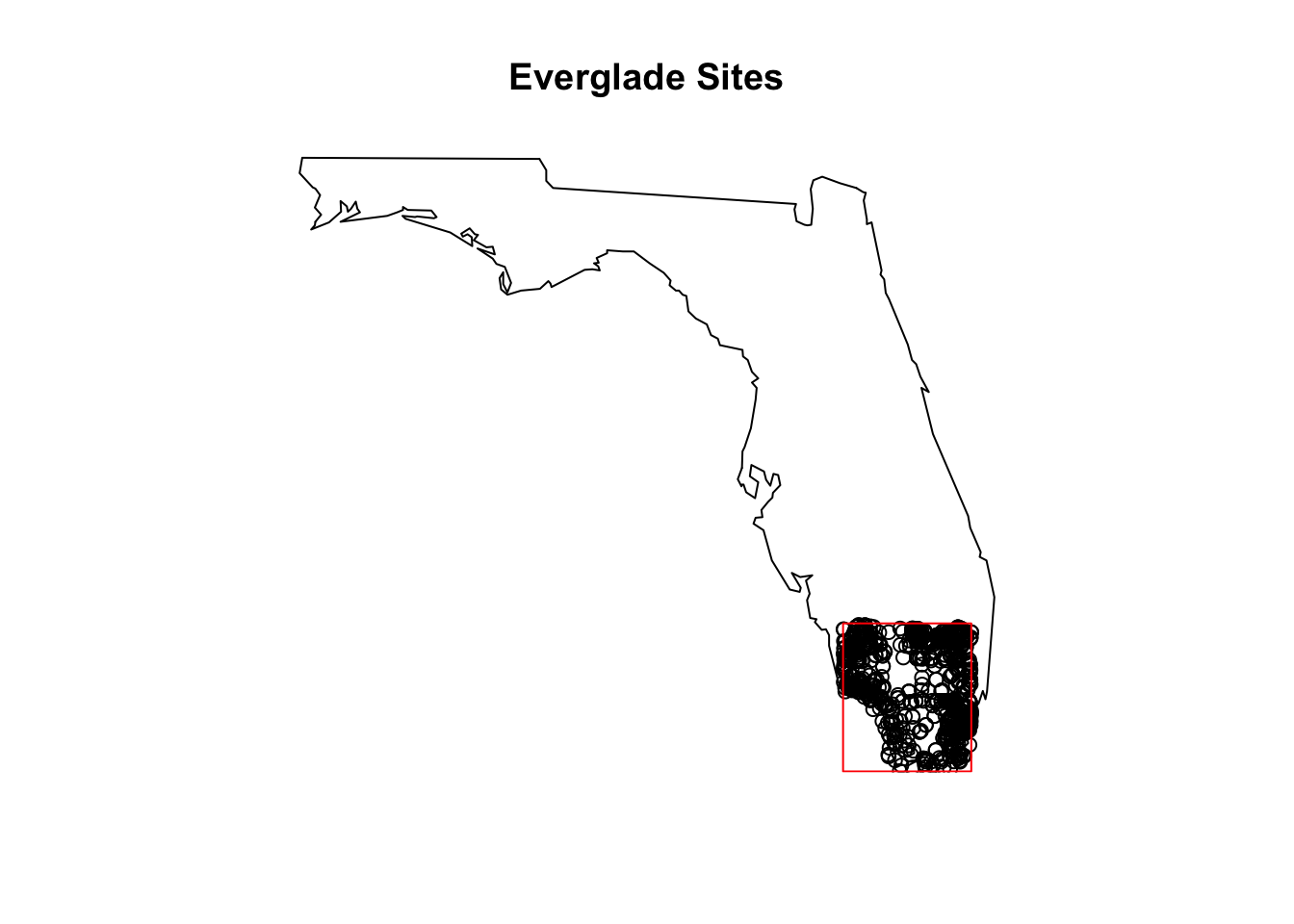
Figure 8.1: A map of NWIS site locations in the Everglades
You can now find and download Water Quality Portal data from R!
8.15 USGS Coding Lab Exercises
8.15.1 Just how dry was the 2020 monsoon?
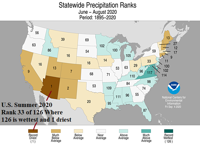
Recently NOAA published a press release demonstrating that 2020 was both the hottest and driest summer on record for Arizona. In this lab we will look at USGS NWIS stream gauge and preciptitation data to investigate just how anomalous 2020 data are.
1: Use the readNWISstat function to retrieve the following statewide data for 2015-2020:
1. Precipitation total (inches/week)
2. Streamflow (ft^3/s)
2: Create two timeseries plots (one for preciptitation, one for streamflow), where color is a function of year (e.g. the x axis is month, the y axis is precipitation, legend shows color by year).
3. Calculate the monthly mean precipitation and streamflow from 2015-2019, and use that mean to calculate a 2020 anomaly timeseries. Create two new plots (like #2 above) with the 2015-2019 mean as a thick black line, and 2020 anomaly as a thin red line.
8.16 geoKnife - Introduction
8.17 Lesson Summary
This lesson will explore how to find and download large gridded datasets via the R package geoknife. The package was created to allow easy access to data stored in the Geo Data Portal (GDP), or any gridded dataset available through the OPeNDAP protocol DAP2 that meets some basic metadata requirements. geoknife refers to the gridded dataset as the fabric, the spatial feature of interest as the stencil, and the subset algorithm parameters as the knife (see below).

figure illustrating definitions of fabric, stencil, and knife
8.18 Lesson Objectives
Explore and query large gridded datasets for efficient and reproducible large-scale analyses.
By the end of this lesson, the learner will be able to:
- Explain the differences between remote and local processing.
- Differentiate the three main concepts of this package: fabric, stencil, and knife.
- Use this package to retrieve pre-processed data from the Geo Data Portal (GDP) via geoknife.
8.19 Lesson Resources
- Publication: geoknife: reproducible web-processing of large gridded datasets
- Tutorial (vignette): geoknife vignette
- An overview of remote processing basics with the Geo Data Portal
- A blog post on visualizing Tropical Storm Colin rainfall with geoknife
- Source code: geoknife on GitHub
- Report a bug or suggest a feature: geoknife issues on GitHub
8.20 Remote processing
The USGS Geo Data Portal is designed to perform web-service processing on large gridded datasets. geoknife allows R users to take advantage of these services by processing large data, such as data available in the GDP catalog or a user-defined dataset, on the web. This type of workflow has three main advantages:
- it allows the user to avoid downloading large datasets,
- it avoids reinventing the wheel for the creation and optimization of complex geoprocessing algorithms, and
- computing resources are dedicated elsewhere, so geoknife operations do not have much of an impact on a local computer.
8.21 geoknife components: fabric, stencil, knife
The main components of a geoknife workflow are the “fabric”, “stencil”, and “knife”. These three components go into the final element, the geoknife “job” (geojob), which defines what the user needs from the processing, allows tracking of the processing status, and methods to dowload the results. The fabric is the gridded web dataset to be processed, the stencil is the feature of interest, and the knife is the processing algorithm parameters. Each of the geoknife components is created using a corresponding function: fabrics are created using webdata(), stencils are created using webgeom() or simplegeom(), and knives are created using webprocess().
This lesson will focus on discovering what options exist for each of those components. The next lesson will teach you how to construct each component and put it together to get the processed data. Before continuing this lesson, load the geoknife library (install if necessary).
## Warning: package 'geoknife' was built under R version 3.6.2##
## Attaching package: 'geoknife'## The following object is masked from 'package:dplyr':
##
## id## The following object is masked from 'package:stats':
##
## start## The following object is masked from 'package:graphics':
##
## title## The following object is masked from 'package:base':
##
## url8.22 Available webdata
8.22.1 GDP datasets
To learn what data is available through GDP, you can explore the online catalog or use the function query. Note that the access pattern for determining available fabrics differs slightly from stencils and knives. Running query("webdata") will return every dataset available through GDP:
## An object of class "datagroup":
## [1] 4km Monthly Parameter-elevation Regressions on Independent Slopes Model Monthly Climate Data for the Continental United States. August 2018 Snapshot
##   url: https://cida.usgs.gov/thredds/dodsC/prism_v2
## [2] 4km Monthly Parameter-elevation Regressions on Independent Slopes Model Monthly Climate Data for the Continental United States. January 2012 Shapshot
##   url: https://cida.usgs.gov/thredds/dodsC/prism
## [3] ACCESS 1980-1999
##   url: https://cida.usgs.gov/thredds/dodsC/notaro_ACCESS_1980_1999
## [4] ACCESS 2040-2059
##   url: https://cida.usgs.gov/thredds/dodsC/notaro_ACCESS_2040_2059
## [5] ACCESS 2080-2099
##   url: https://cida.usgs.gov/thredds/dodsC/notaro_ACCESS_2080_2099
## [6] Bias Corrected Constructed Analogs V2 Daily Future CMIP5 Climate Projections
## url: https://cida.usgs.gov/thredds/dodsC/cmip5_bcca/future## [1] 532Notice that the object returned is a special geoknife class of datagroup. There are specific geoknife functions that only operate on an object of this class, see ?title and ?abstract. These two functions are used to extract metadata information about each of the available GDP datasets. With 532 datasets available, it is likely that reading through each to find ones that are of interest to you would be time consuming. You can use grep along with the functions title and abstract to figure out which datasets you would like to use for processing.
Let’s say that we were interested in evapotranspiration data. To search for which GDP datasets might contain evapotranspiration data, you can use the titles and abstracts.
# notice that you cannot perform a grep on all_webdata - it is because it is a special class
# `grep("evapotranspiration", all_webdata)` will fail
# you need to perform pattern matching on vectors

all_titles <- title(all_webdata)
which_titles <- grep("evapotranspiration", all_titles)
evap_titles <- all_titles[which_titles]
head(evap_titles)
## [1] "Monthly Conterminous U.S. actual evapotranspiration data"
## [2] "Yearly Conterminous U.S. actual evapotranspiration data"all_abstracts <- abstract(all_webdata)
which_abstracts <- grep("evapotranspiration", all_abstracts)
evap_abstracts <- all_abstracts[which_abstracts]
evap_abstracts[1]## [1] "Reference evapotranspiration (ET0), like potential evapotranspiration, is a measure of atmospheric evaporative demand. It was used in the context of this study to evaluate drought conditions that can lead to wildfire activity in Alaska using the Evaporative Demand Drought Index (EDDI) and the Standardized Precipitation Evapotranspiration Index (SPEI). The ET0 data are on a 20km grid with daily temporal resolution and were computed using the meteorological inputs from the dynamically downscaled ERA-Interim reanalysis and two global climate model projections (CCSM4 and GFDL-CM3). The model projections are from CMIP5 and use the RCP8.5 scenario. The dynamically downscaled data are available at https://registry.opendata.aws/wrf-alaska-snap/. The ET0 was computed following the American Society of Civil Engineers Standardized Reference Evapotranspiration Equation based on the downscaled daily temperature, humidity and winds. The full details of the computation of ET0, an evaluation of the underlying data, and the assessment of the fire indices are described in Ziel et al. (2020; https://doi.org/10.3390/f11050516)."13 possible datasets to look through is a lot more manageable than 532. Let’s say the dataset titled “Yearly Conterminous U.S. actual evapotranspiration data” interested us enough to explore more. We have now identified a fabric of interest.
We might want to know more about the dataset, such as what variables and time periods are available. To actually create the fabric, you will need to use webdata and supply the appropriate datagroup object as the input. This should result in an object with a class of webdata. The following functions will operate only on an object of class webdata.
evap_fabric <- webdata(all_webdata["Yearly Conterminous U.S. actual evapotranspiration data"])
class(evap_fabric)
## [1] "webdata"
## attr(,"package")
## [1] "geoknife"Now that we have a defined fabric, we can explore what variables and time period are within that data. First, we use query to determine what variables exist. You’ll notice that the function variable returns NA. This is fine when you are just exploring available data; however, exploring available times requires that the variable be defined because sometimes individual variables within a dataset can have different time ranges. Thus, we need to set which variable from the dataset will be used. Then, we can explore times that are available in the data. Using query() is helpful when exploring datasets, but is unecessary if you already know what times and variables you’d like to access.
## [1] NA## [1] "et"# trying to find available times before setting the variable results in an error
# `query(evap_fabric, "times")` will fail
# only one variable, "et"
variables(evap_fabric) <- "et"
variables(evap_fabric)## [1] "et"## [1] "2000-01-01 UTC" "2018-01-01 UTC"8.22.2 Datasets not in GDP
Any gridded dataset available online that follows OPeNDAP protocol and some additional conventions can be used with geoknife. These datasets can be found through web searches or other catalogs and require finding out the OPeNDAP endpoint (URL) for the dataset. This url is used as the input to the argument url in webdata. Please email the GDP development team (gdp@usgs.gov) with questions abvout these specifics.
There are hundreds (or potentially thousands) of additional OPeNDAP datasets that will work with geoknife, but need to be found through web searches or catalogs (e.g., www.esrl.noaa.gov/psd/thredds/dodsC/Datasets and apdrc.soest.hawaii.edu/data/data.php ).
We searched NOAA’s OPenDAP data catalog and found data from the Center for Operational Oceanographic Products and Services THREDDS server. It includes forecasts for water levels, water currents, water temperatures, and salinity levels for Delaware Bay. Since it is forecasted data, the times associated with the data will change. To create a webdata object from this dataset, just use the OPeNDAP url. Then query variables and time as we did before.
DelBay_fabric <- webdata(url="https://opendap.co-ops.nos.noaa.gov/thredds/dodsC/DBOFS/fmrc/Aggregated_7_day_DBOFS_Fields_Forecast_best.ncd")
query(DelBay_fabric, "variables")
## [1] "zeta" "u" "v" "w" "temp" "Pair" "Uwind" "Vwind" "h"
## [10] "f" "pm" "pn" "angle"# need to set the variable(s) in order to query the times
variables(DelBay_fabric) <- "temp"
query(DelBay_fabric, "times")## [1] "2021-02-04 UTC" "2021-02-14 UTC"The first example we’ve included here uses aggregated data, meaning there is a single URL for all the data of this type on the server. Some data that you encounter might be non-aggregated, meaning there are multiple URLs to access the same data. In these cases, you will need to create more than one geojob and join data at the end.
Here is a second example of using a non-GDP dataset which is not aggregated in times or variables. This data was found under the data section on Unidata’s THREDDS server. This example includes water vapor at 8km resolution at national extent from here.
wv_fabric <- webdata(url="https://thredds.ucar.edu/thredds/dodsC/satellite/WV/SUPER-NATIONAL_8km/current/SUPER-NATIONAL_8km_WV_20200904_1330.gini")
query(wv_fabric, "variables")
## [1] "IR_WV"# need to set the variable(s) in order to query the times
variables(wv_fabric) <- "IR_WV"
query(wv_fabric, "times") # Note the times of this dataset include only a single timestep, since the data collection has a file for each time## [1] "2020-09-04 UTC" "2020-09-04 UTC"The url used here for webdata() contains the date and the time, so we would need to construct a loop through multiple timesteps in order to assemble a time series from this data source.
8.23 Available webgeoms
Now that we have explored options for our webdata, let’s look at what options exist for geospatial features.
The next component to geoknife jobs is the spatial extent of the data, a.k.a. the stencil. The stencil is defined by using either of the functions simplegeom or webgeom. simplegeom is used to explicitly define an area by the user, but webgeom is used to specify an existing web feature service (WFS) as the geospatial extent. Defining your stencil using simplegeom will be covered in the next lesson. This lesson will just show you how to learn what available webgeoms exist. Users can use any WFS url to create their stencil, but there are a number of features that exist through GDP already. To determine what features exist, you can create a default webgeom object and then query its geom name, attributes, and values. This will return all available GDP default features.
# setup a default stencil by using webgeom and not supplying any arguments
default_stencil <- webgeom()

# now determine what geoms are available with the default
default_geoms <- query(default_stencil, "geoms")
length(default_geoms)
## [1] 75## [1] "upload:Ag_Lands_ICC"
## [2] "upload:Ag_Lands_ICC_ForOnlineProcesses"
## [3] "upload:Ag_Lands_Reservation"
## [4] "upload:Airport_Polygon"
## [5] "sample:Alaska"
## [6] "upload:BBShapefile"You will notice a pattern with the names of the geoms: a category followed by :, and then a specific name. These category-name combinations are the strings you would use to define your geom. Additionally, webgeom can accept a URL that points directly to a WFS. The categories you should be familiar with are sample and upload. sample geoms are any that are available through geoknife by default. upload geoms are custom shapefiles that someone uploaded through GDP. If you would like to upload a specific shapefile to GDP, go to the advanced spatial section in GDP. Be aware that uploaded shapefiles are wiped from the server at regular intervals (could be as often as weekly). To use your own shapefile: upload it as a zip shapefile, execute your job and then save the output; re-upload your shapefile the next time you need it on GDP if it has expired.
Similar to fabrics where you could not query times without setting the variables, you cannot query attributes of stencils before defining the geoms. Likewise, you cannot query for values of a stencil until you have set the attributes. Attributes give the metadata associated with the stencil and it’s geom. Values tell you the individual spatial features available in that attribute of the geom.
## [1] NAgeom(default_stencil) <- "sample:CONUS_states"
# now that geom is set, you can query for available attributes
query(default_stencil, "attributes")## [1] "STATE" "FIPS"attribute(default_stencil) <- "STATE"
# now that attribute is set, you can query for available values
STATE_values <- query(default_stencil, "values")
head(STATE_values)## [1] "Alabama" "Arizona" "Arkansas" "California" "Colorado"
## [6] "Connecticut"# switch the stencil to see the differences
ecoreg_stencil <- default_stencil
geom(ecoreg_stencil) <- "sample:Ecoregions_Level_III"
query(ecoreg_stencil, "attributes")## [1] "LEVEL3_NAM"attribute(ecoreg_stencil) <- "LEVEL3_NAM"
ecoreg_values <- query(ecoreg_stencil, "values")
head(ecoreg_values)## [1] "Ahklun And Kilbuck Mountains" "Alaska Peninsula Mountains"
## [3] "Alaska Range" "Aleutian Islands"
## [5] "Arctic Coastal Plain" "Arctic Foothills"# now set the values to the Driftless Area and Blue Ridge ecoregions
values(ecoreg_stencil) <- ecoreg_values[c(12, 33)]
values(ecoreg_stencil)## [1] "Blue Ridge" "Driftless Area"There are some built-in templates that allow stencils to be defined more specifically. Currently, the package only supports US States, Level III Ecoregions, or HUC8s. Below are shortcuts to setting the geom, attribute, and values.
## An object of class "webgeom":
## url: https://cida.usgs.gov/gdp/geoserver/wfs
## geom: sample:CONUS_states
## attribute: STATE
## values: Wisconsin
## wfs version: 1.1.0## An object of class "webgeom":
## url: https://cida.usgs.gov/gdp/geoserver/wfs
## geom: sample:CONUS_states
## attribute: STATE
## values: Wisconsin, Maine
## wfs version: 1.1.0## An object of class "webgeom":
## url: https://cida.usgs.gov/gdp/geoserver/wfs
## geom: sample:simplified_huc8
## attribute: HUC_8
## values: 09020306, 14060009
## wfs version: 1.1.0## An object of class "webgeom":
## url: https://cida.usgs.gov/gdp/geoserver/wfs
## geom: sample:Ecoregions_Level_III
## attribute: LEVEL3_NAM
## values: Colorado Plateaus, Driftless Area
## wfs version: 1.1.08.24 Available webprocesses
The final component to a geojob is the process algorithm used to aggregate the data across the defined stencil. Web process algorithms can be defined by the user, but let’s explore the defaults available through GDP.
# setup a default knife by using webprocess and not supplying any arguments
default_knife <- webprocess()

# now determine what web processing algorithms are available with the default
default_algorithms <- query(default_knife, 'algorithms')
length(default_algorithms)
## [1] 6## $`Timeseries Service Subset`
## [1] "gov.usgs.cida.gdp.wps.algorithm.FeatureTimeSeriesAlgorithm"
##
## $`Categorical Coverage Fraction`
## [1] "gov.usgs.cida.gdp.wps.algorithm.FeatureCategoricalGridCoverageAlgorithm"
##
## $`OPeNDAP Subset`
## [1] "gov.usgs.cida.gdp.wps.algorithm.FeatureCoverageOPeNDAPIntersectionAlgorithm"
##
## $`Area Grid Statistics (unweighted)`
## [1] "gov.usgs.cida.gdp.wps.algorithm.FeatureGridStatisticsAlgorithm"
##
## $`Area Grid Statistics (weighted)`
## [1] "gov.usgs.cida.gdp.wps.algorithm.FeatureWeightedGridStatisticsAlgorithm"
##
## $`WCS Subset`
## [1] "gov.usgs.cida.gdp.wps.algorithm.FeatureCoverageIntersectionAlgorithm"From this list, you can define which algorithm you would like the webprocess component to use. Definitions of each of the default algorithms can be found in the Geo Data Portal Algorithm Summaries section of the GDP process documentation. For example, we want to use the OPeNDAP subsetting algorithm, “OPeNDAP Subset”, which downloads a spatiotemporal chunk of data without any spatial processing.
## $`Area Grid Statistics (weighted)`
## [1] "gov.usgs.cida.gdp.wps.algorithm.FeatureWeightedGridStatisticsAlgorithm"# change the algorithm to OPeNDAP's subset
algorithm(default_knife) <- default_algorithms['OPeNDAP Subset']
algorithm(default_knife)## $`OPeNDAP Subset`
## [1] "gov.usgs.cida.gdp.wps.algorithm.FeatureCoverageOPeNDAPIntersectionAlgorithm"Now that we can explore all of our options, we will learn how to construct each component and execute a geojob in the next lesson.
8.25 Setting up a geojob
A geojob is the object that contains all of the necessary processing information to execute a data request to GDP. The geojob is made up of the stencil, fabric, and knife.
To create a geojob, use the function geoknife and give the three components as arguments. stencil and fabric must be indicated, but knife has a default. Any additional arguments are specifications for the webprocessing step. See ?'webprocess-class' for options. This portion of the lesson will not discuss all of the options.
Let’s setup a geojob to find the unweighted annual evapotranspiration rates for the state of Indiana using the annual evapotranspiration data we saw in the previous section. Since we have seen the URL and know the available variables and times, we can set all of that directly in the webdata function. Note: the times field must be a vector of start then end date, and be class POSIXct or character.
# create fabric
evap_fabric <- webdata(times = c("2005-01-01", "2015-01-01"),
                         variables = "et",
                         url = 'https://cida.usgs.gov/thredds/dodsC/ssebopeta/yearly')

# create stencil
evap_stencil <- webgeom('state::Indiana')

# create knife (which defaults to weighted)
evap_knife <- webprocess()
# find unweighted algorithm
all_algorithms <- query(evap_knife, 'algorithms')
unw_algorithm <- all_algorithms[grep('unweighted', names(all_algorithms))]
# set knife algorithm to unweighted
algorithm(evap_knife) <- unw_algorithm

# create the geojob
evap_geojob <- geoknife(evap_stencil, evap_fabric, evap_knife)
8.26 Checking the geojob status
The geojob has been created and started on the server. Now, you can check to see if the processing is complete by using check.
## $status
## [1] "Process successful"
##
## $URL
## [1] "https://cida.usgs.gov:443/gdp/process/RetrieveResultServlet?id=090e2f71-9735-453d-9bf0-0a3b266c9f72OUTPUT"
##
## $statusType
## [1] "ProcessSucceeded"
##
## $percentComplete
## [1] "100"
Other helpful functions to get status information about the job are running (returns TRUE/FALSE to say if the job is still processing), error (returns TRUE/FALSE to say if there was an error during the processing), and successful (returns TRUE/FALSE indicating whether the job process was able to complete without any issues). Only one of these can return TRUE at a time.
## [1] FALSE## [1] FALSE## [1] TRUEThe results of all the status checks say that our job was successful. These status checks are useful if you put a geojob in a script and want to fail gracefully when there is an error in the job.
8.27 Getting geojob data
Since this job has finished processing and was successful, you can now get the data. You’ll notice that evap_geojob does not actually contain any data. It only contains information about the job that you submitted. To get the data, you need to use result or download. The feature summary algorithms will return simple tabular data, so you can use result to automatically take the output and parse it into an R data.frame. We used a feature summary algorithm in the evapotranspiration example, which returned tabular data. So, let’s use result to get the geojob output.
## [1] 11## DateTime Indiana variable statistic
## 1 2005-01-01 603.7376 et MEAN
## 2 2006-01-01 688.1866 et MEAN
## 3 2007-01-01 576.3254 et MEAN
## 4 2008-01-01 691.2009 et MEAN
## 5 2009-01-01 689.2706 et MEAN
## 6 2010-01-01 630.4045 et MEANThere are additional algorithms that return subsets of the raw data as netcdf or geotiff formats. These formats will require you to handle the output manually using download. Use this function to download the output to a file and then read it using your preferred data parsing method. download can also be used for tabular data if you have a parsing method that differs from what is used in result. See ?download for more information.
8.28 wait and email
This was not a computationally or spatially intensive request, so the job finished almost immediately. However, if we had setup a more complex job, it could still be running. Even though the processing of these large gridded datasets uses resources on a remote server, your workflow needs to account for processing time before using the results. There are a few scenarios to consider:
- You are manually executing a job and manually checking it.
- You are running a script that kicks off a
geoknifeprocess followed by lines of code that use the returned data. - You are running a long
geoknifeprocess and want to be able to close R/RStudio and come back to a completed job later.
For the first scenario, the workflow from above was fine. If you are manually checking that the job has completed before trying to extract results, then nothing should fail.
For the second scenario, your code will fail because it will continue to execute the code line by line after starting the job. So, your code will fail at the code that gets the data (result/download) since the job is still running. You can prevent scripts from continuing until the job is complete by using the function wait. This function makes a call to GDP at specified intervals to see if the job is complete, and allows the code to continue once the job is complete. This function has two arguments: the geojob object and sleep.time. sleep.time defines the interval at which to check the status of the job in seconds (the default for sleep.time is 5 seconds). Please try to adjust sleep.time to limit the number of calls to GDP, e.g. if you know the job will take about an hour, set sleep.time=120 (2 min) because every 5 seconds would be excessive.
# typical wait workflow
evap_geojob <- geoknife(evap_stencil, evap_fabric, evap_knife)
wait(evap_geojob, sleep.time = 20)
evap_data <- result(evap_geojob)
If you know ahead of time that your process will be long, you can tell the job to wait when defining your knife (the default is to not wait). sleep.time can be specified as an argument to webprocess. The following is functionally the same as the use of wait() from above.
# create knife with the args wait and sleep.time
evap_knife <- webprocess(wait=TRUE, sleep.time=20)

# follow the same code from before to get the unweighted algorithm
all_algorithms <- query(evap_knife, 'algorithms')
unw_algorithm <- all_algorithms[grep('unweighted', names(all_algorithms))]
algorithm(evap_knife) <- unw_algorithm

# create geojob using knife w/ wait
evap_geojob <- geoknife(evap_stencil, evap_fabric, evap_knife)

# get result
evap_data <- result(evap_geojob)
As for the third scenario, if you have a job that will take a long time and plan to close R in the interim, you can specify the argument email when creating the knife. Then when you use your new knife in the geoknife call, it will send an email with appropriate information upon job completion (you will see gdp_data@usgs.gov as the sender).
# example of how to specify an email address to get a job completion alert
knife_willemail <- webprocess(email='fake.email@gmail.com')
knife_willemail
## An object of class "webprocess":
## url: https://cida.usgs.gov/gdp/process/WebProcessingService
## algorithm: Area Grid Statistics (weighted)
## web processing service version: 1.0.0
## process inputs:
## SUMMARIZE_TIMESTEP: false
## SUMMARIZE_FEATURE_ATTRIBUTE: false
## DELIMITER: COMMA
## REQUIRE_FULL_COVERAGE: true
## STATISTICS:
## GROUP_BY:
## wait: FALSE
## email: fake.email@gmail.comThe email alert will contain the completed job URL. Since this process requires you to leave R and get information from an email, it is often only recommended if you don’t plan to do further analysis in R, or you use saveRDS to save the geojob object so you can load it in a later session. Otherwise, we recommend using the wait() function in a script. Use the URL as a string in this workflow to get your results:
8.29 Putting it all together, mapping precipitation from Tropical Storm Colin
The following example is slightly modified from the blog post here and shows a workflow for accessing rainfall data for the time period covering Tropical Storm Colin and visualizing the total rainfall per county during the time range.
Define a function to retrieve precip data using geoknife
getPrecip <- function(states, startDate, endDate){

    # use fips data from maps package
    counties_fips <- maps::county.fips %>%
        mutate(statecounty=as.character(polyname)) %>% # character to split into state & county
        tidyr::separate(polyname, c('statename', 'county'), ',') %>%
        mutate(fips = sprintf('%05d', fips)) %>% # fips need 5 digits to join w/ geoknife result
        filter(statename %in% states)

    stencil <- webgeom(geom = 'sample:Counties',
                       attribute = 'FIPS',
                       values = counties_fips$fips)

    fabric <- webdata(url = 'https://cida.usgs.gov/thredds/dodsC/UofIMETDATA',
                      variables = "precipitation_amount",
                      times = c(startDate, endDate))

    job <- geoknife(stencil, fabric, wait = TRUE, REQUIRE_FULL_COVERAGE=FALSE)
    check(job)
    precipData_result <- result(job, with.units=TRUE)
    precipData <- precipData_result %>%
        select(-variable, -statistic, -units) %>%
        gather(key = fips, value = precipVal, -DateTime) %>%
        left_join(counties_fips, by="fips") #join w/ counties data

    return(precipData)

}
# Function to map cumulative precipitation data using R package maps:
precipMap <- function(precipData, startDate, endDate){
  cols <- colorRampPalette(brewer.pal(9,'Blues'))(9)
  precip_breaks <- c(seq(0,80,by = 10), 200)

  precipData_cols <- precipData %>%
    group_by(statename, statecounty) %>%
    summarize(cumprecip = sum(precipVal)) %>%
    mutate(cols = cut(cumprecip, breaks = precip_breaks, labels = cols, right=FALSE)) %>%
    mutate(cols = as.character(cols))

  par(mar = c(0,0,3,0))

  map('county', regions = precipData_cols$statecounty,
      fill = TRUE, col = precipData_cols$cols, exact=TRUE)

  legend(x = "bottomright", fill = cols, cex = 0.7, bty = 'n',
         title = "Cumulative\nPrecipitation (mm)",
         legend = c(paste('<', precip_breaks[-c(1,length(precip_breaks))]),
                    paste('>', tail(precip_breaks,2)[1]))) # greater
  graphics::title("Cumulative Precipitation from Tropical Storm Colin",
                  line = 2, cex.main=1.2)  #title was being masked by geoknife
  mtext(side = 3, line = 1, cex = 0.9,
        text= paste("By county from", startDate, "to", endDate))
}

# Now, we can use those functions to fetch data for specific counties and time periods.
# TS Colin made landfall on June 6th and moved into open ocean on June 7th. Use these dates as the start and end times in our
# function (need to account for timezone, +5 UTC). We can visualize the path of the storm by mapping cumulative precipitation for each county.
library(dplyr)
library(tidyr)
library(geoknife) #order matters because 'query' is masked by a function in dplyr
library(RColorBrewer)
library(maps)

statesTSColin <- c('florida', 'alabama', 'georgia',
                   'south carolina', 'north carolina')
startTSColin <- "2016-06-06 05:00:00"
endTSColin <- "2016-06-08 05:00:00"

precipData <- getPrecip(states = statesTSColin,
                        startDate = startTSColin,
                        endDate = endTSColin)
precipMap(precipData,
          startDate = startTSColin,
          endDate = endTSColin)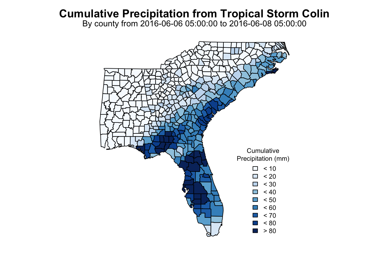
8.30 USGS NWIS Culmination Write Up
Write up a 1-page derived data product or research pipeline proposal summary of a project that you might want to explore using USGS NWIS and USGS GDP data. Include the types of data that you would need to implement this project and how you would retrieve them. Save this summary as you will be refining and adding to your ideas over the course of the semester.
Suggestions:
Tables or bullet lists of specific data products
An overarching high-quality figure to show how these data align
One paragraph summarizing how this data or analysis is useful to you and/or the infrastructure.