Chapter 4 PhenoCam: Digital Repeat Photography Networks & Methods
Estimated Time: 4 hours
Course participants: As you review this information, please consider the final course project that you will work on at the over this semester. At the end of this section, you will document an initial research question or idea and associated data needed to address that question, that you may want to explore while pursuing this course.
4.1 Digital Repeat Photography Networks Learning Objectives
At the end of this activity, you will be able to:
Understand how phenology is a large driver of biosphere-atmosphere interactions, and is a sensitive indicator of climate change.
Summarize data which can be pulled out of digital repeat imagery
Describe basic processing of digital repeat photography
Perform basic image processing.
Estimate image haziness as an indication of fog, cloud or other natural or artificial factors using the
hazerR package.Define and use a Region of Interest, or ROI, for digitial repeat photography methods.
Handle Field-of-View (FOV) shifts in digital repeat photography.
Extract timeseries data from a stack of images using color-based metrics.
4.2 The PhenoCam Network Mission & Design
Since its inception, the objective of the PhenoCam network has been to serve as a repository for phenologically-relevant, digital, repeat (time-lapse) imagery, and to make that imagery, and derived data products, freely available to a wide array of third-party data end-users, including researchers, educators, and the general public.
“Thus, imagery from the PhenoCam archive is made publicly available, without restriction, and we encourage you to download imagery and datasets for use in your own research and teaching. In return, we ask that you acknowledge the source of the data and imagery, and abide by the terms of the Creative Commons CC BY Attribution License.”
4.2.1 Relevant documents & background information:
4.3 PhenoCam’s Spatial design:
The PhenoCam Network is:
A voluntary ‘opt in’ network with collaborators who are varied, including:
Individual research labs or field sites in North America, Europe, Asia, Africa, South America
Individuals who think it would be cool to be part of a network like this
The project is largely run by the Richardson Lab at NAU, with support from key collaborators at the University of New Hampshire who provide server and website management.
Anyone can buy a relatively inexpensive camera, run some simple scripts to correct for things like auto-white balance (which we will cover later), and patch in to the netowrk. PhenoCam then retrieves, archieves and processess imagery for distribution.
4.3.1 PhenoCam as a Near Surface Remote Sensing Technique
6 years of PhenoCam imagery at Harvard Forest
PhenoCam uses imagery from networked digital cameras for continuous monitoring of plant canopies
Images are recorded approximately every 30 minutes (every 15 minutes for NEON), sunrise to sunset, 365 days a year
The scale of observations is comparable to that of tower-based land-atmosphere flux measurements
PhenoCams provide a direct link between what is happening on the ground and what is seen by satellites PhenoCams cover a wide array of:
Plant Funtional Types (PFTs)
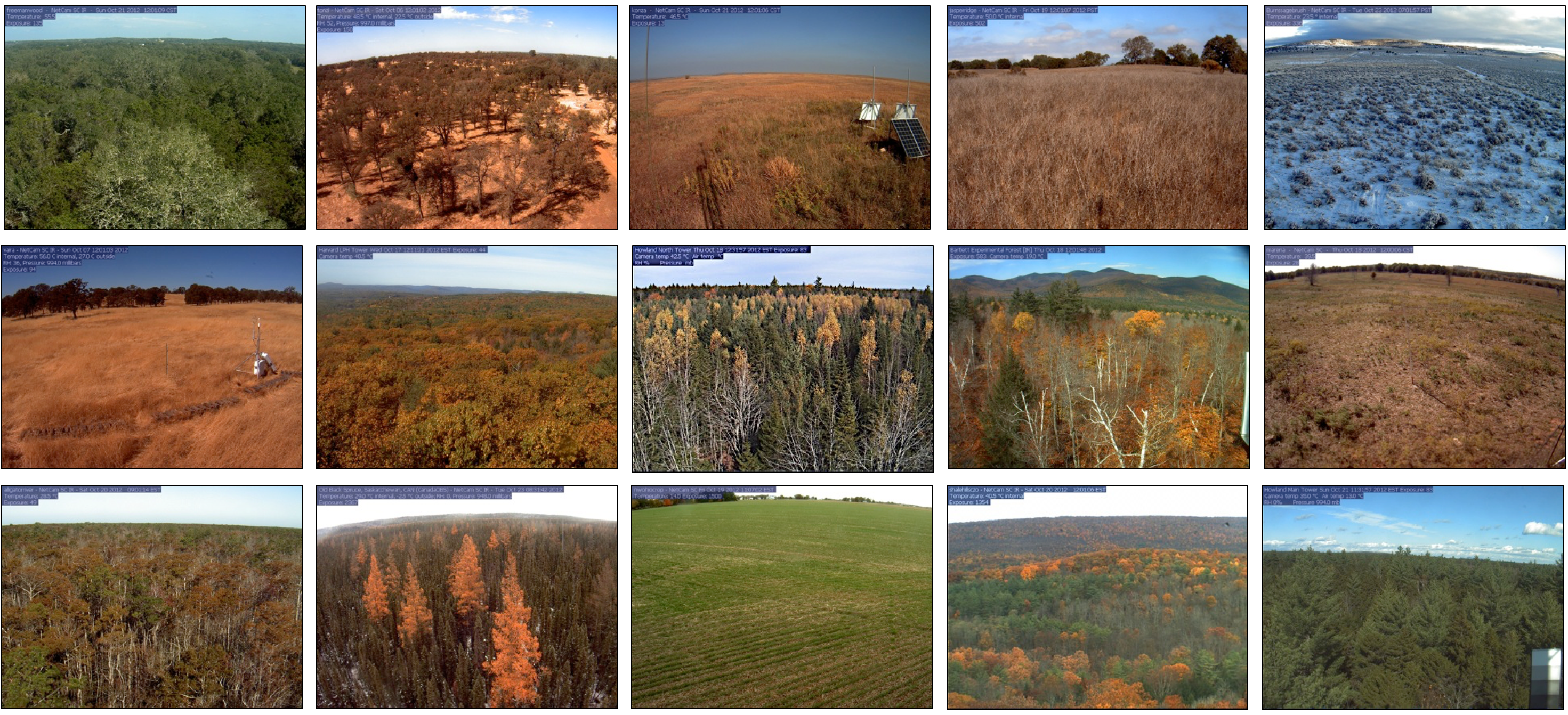
- Ecoregions
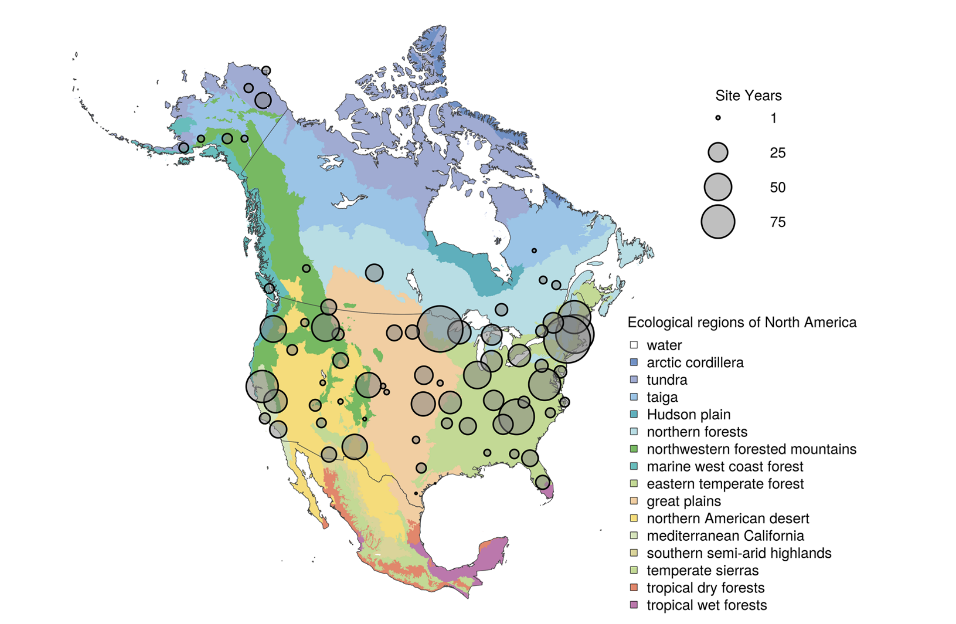
Spatial distribution of PhenoCam data across ecological regions of North America. Background map illustrates USA Environmental Protection Agency Level I Ecoregions. Data counts have been aggregated to a spatial resolution of 4°, and the size of each circle corresponds to the number of site-years of data in the 4×4° grid cell. Sites in Hawaii, Puerto Rico, Central and South America, Europe, Asia and Africa (total of 88 site years) are not shown. (Seyednasrollah et al., 2019)
Co-Located Networks
Ambient vs. Experimental set ups
4.3.2 How PhenoCams Pull Data
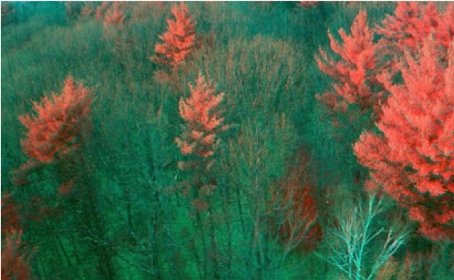
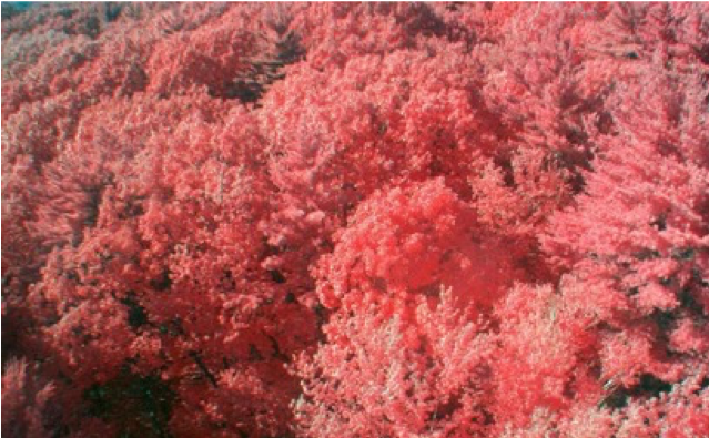
4.3.3 Leveraging camera near-infrared (NIR) capabilities
Petach et al., Agricultural & Forest Meteorology 2014
CMOS sensor is sensitive to > 700 nm
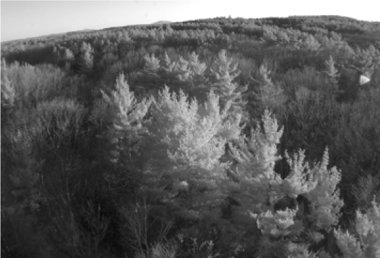
A software-controlled filter enables sequential VIS (RGB color) and VIS+NIR (monochrome) images Potential applications:
false color images
“camera NDVI” as alternative to GCC
4.4 Digital Repeat Photography Written Questions
Suggested completion: Before Digital Repeat Photography methods (day 2 PhenoCam)
Question 1: What do you see as the value of the images themselves? The 1 or 3-day products, the transition dates? How could they be used for different applications?
Question 2: Why does PhenoCam take photos every 15-30 minutes, but summarize to 1 or 3-day products?
Question 3: Why does canopy color coordiante with photosynthesis in many ecosystems? Name an example of a situation where it wouldn’t and explain why.
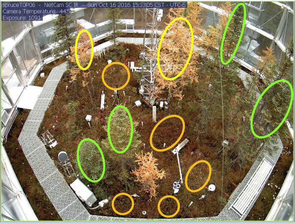
Question 4: Why are there sometimes multiple Regions of Interest (ROIs) for a PhenoCam?
Question 5: How might or does the PhenoCam project intersect with your current research or future career goals? (1 paragraph)
Question 6: Use the map on the PhenoCam website to answer the following questions. Consider the research question that you may explore as your final semester project or a current project that you are working on and answer each of the following questions:
- Are there PhenoCams that are in study regions of interest to you?
- Which PhenoCam sites does your current research or final project ideas
coincide with?
- Are they connected to other networks (e.g. LTAR, NEON, Fluxnet)?
- What is the data record length for the sites you’re interested in?
Question 7: Consider either your current or future research, or a question you’d like to address durring this course:
- Which types of PhenoCam data may be more useful to address these questions?
- What non-PhenoCam data resources could be combined to help address your question?
- What challenges, if any, could you foresee when beginning to work with these data?
4.5 Introduction to Digital Repeat Photography Methods
The concept of repeat photography for studying environmental has been introduced to scientists long time ago (See Stephens et al., 1987). But in the past decade the idea has gained much popularity for monitoring environmental change (e.g., Sonnentag et al., 2012). One of the main applications of digital repeat photography is studying vegetation phenology for a diverse range of ecosystems and biomes (Richardson et al., 2019). The methods has also shown great applicability in other fields such as:
assessing the seasonality of gross primary production,
salt marsh restoration,
monitoring tidal wetlands,
investigating growth in croplands, and
evaluating phenological data products derived from satellite remote sensing.
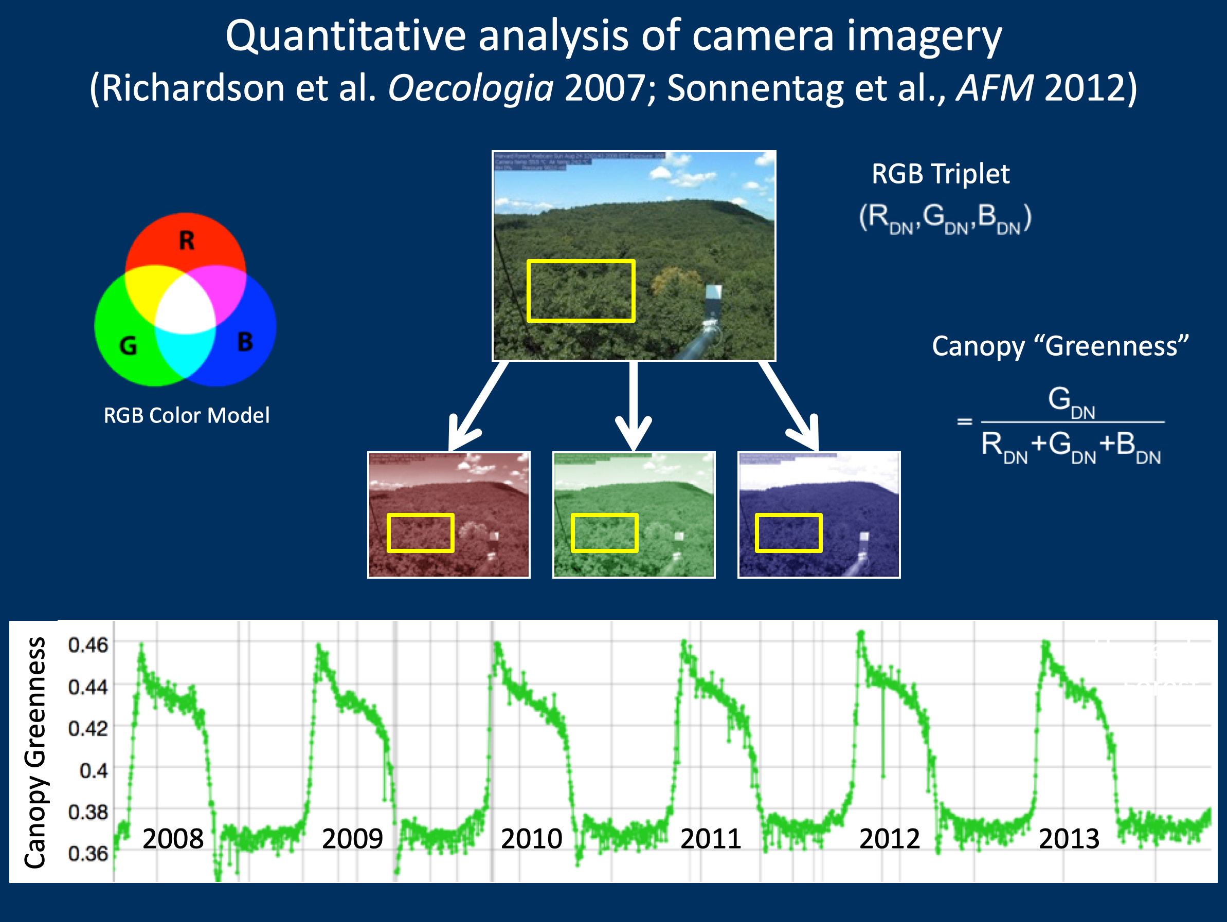
Obtaining quantitative data from digital repeat photography images is usually performed by defining appropriate region of interest, also know as ROI’s, and for the red (R), green (G) and blue (B) color channels, calculating pixel value (intensity) statistics across the pixels within each ROI. ROI boundaries are delineated by mask files which define which pixels are included and which are excluded from these calculations.
The masks are then used to extract color-based time series from a stack of images. Following the time-series, statistical metrics are used to obtain 1-day and 3-day summary time series. From the summary product time series, phenological transition dates corresponding to the start and the end of green-up and green-down phenological phases are calculated. In this chapter we explain this process by starting from general image processing tools and then to phenocam-based software applications.
For more details about digital repeat photogrpahy you can check out the following publications: - Seyednarollah, et al. 2019, “Tracking vegetation phenology across diverse biomes using Version 2.0 of the PhenoCam Dataset”. - Seyednarollah, et al. 2019, “Data extraction from digital repeat photography using xROI: An interactive framework to facilitate the process”.
4.6 Pulling Data via the phenocamapi Package
The phenocamapi R package is developed to simplify interacting with the PhenoCam network dataset and perform data wrangling steps on PhenoCam sites’ data and metadata.
This tutorial will show you the basic commands for accessing PhenoCam data through the PhenoCam API. The phenocampapi R package is developed and maintained by Bijan Seyednarollah. The most recent release is available on GitHub (PhenocamAPI). Additional vignettes can be found on how to merge external time-series (e.g. Flux data) with the PhenoCam time-series.
We begin with several useful skills and tools for extracting PhenoCam data directly from the server:
- Exploring the PhenoCam metadata
- Filtering the dataset by site attributes
- Extracting the list of midday images
- Downloading midday images for a given time range
4.7 Exploring PhenoCam metadata
Each PhenoCam site has specific metadata including but not limited to how a site is set up and where it is located, what vegetation type is visible from the camera, and its climate regime. Each PhenoCam may have zero to several Regions of Interest (ROIs) per vegetation type. The phenocamapi package is an interface to interact with the PhenoCam server to extract those data and process them in an R environment.
To explore the PhenoCam data, we’ll use several packages for this tutorial.
## Loading required package: rjson## Loading required package: RCurl## Warning: package 'RCurl' was built under R version 3.6.2## Warning: package 'lubridate' was built under R version 3.6.2##
## Attaching package: 'lubridate'## The following objects are masked from 'package:data.table':
##
## hour, isoweek, mday, minute, month, quarter, second, wday, week,
## yday, year## The following objects are masked from 'package:base':
##
## date, intersect, setdiff, unionWe can obtain an up-to-date data.frame of the metadata of the entire PhenoCam
network using the get_phenos() function. The returning value would be a
data.table in order to simplify further data exploration.
# obtaining the phenocam site metadata from the server as data.table
phenos <- phenocamapi::get_phenos()

# checking out the first few sites
head(phenos$site)
## [1] "aafcottawacfiaf14e" "aafcottawacfiaf14w" "acadia"
## [4] "aguatibiaeast" "aguatibianorth" "ahwahnee"## [1] "site" "lat"
## [3] "lon" "elev"
## [5] "active" "utc_offset"
## [7] "date_first" "date_last"
## [9] "infrared" "contact1"
## [11] "contact2" "site_description"
## [13] "site_type" "group"
## [15] "camera_description" "camera_orientation"
## [17] "flux_data" "flux_networks"
## [19] "flux_sitenames" "dominant_species"
## [21] "primary_veg_type" "secondary_veg_type"
## [23] "site_meteorology" "MAT_site"
## [25] "MAP_site" "MAT_daymet"
## [27] "MAP_daymet" "MAT_worldclim"
## [29] "MAP_worldclim" "koeppen_geiger"
## [31] "ecoregion" "landcover_igbp"
## [33] "dataset_version1" "site_acknowledgements"
## [35] "modified" "flux_networks_name"
## [37] "flux_networks_url" "flux_networks_description"Now we have a better idea of the types of metadata that are available for the Phenocams.
4.7.1 Remove null values
We may want to explore some of the patterns in the metadata before we jump into specific locations.
Let’s look at Mean Annual Precipitation (MAP) and Mean Annual
Temperature (MAT) across the different field site and classify those by the
primary vegetation type (primary_veg_type) for each site. We can find out what
the abbreviations for the vegetation types mean from the following table:
| Abbreviation | Description |
|---|---|
| AG | agriculture | |
| DB | deciduous broadleaf | |
| DN | deciduous needleleaf | |
| EB | evergreen broadleaf | |
| EN | evergreen needleleaf | |
| GR | grassland | |
| MX | mixed vegetation (generally EN/DN, DB/EN, or DB/EB) | |
| SH | shrubs | |
| TN | tundra (includes sedges, lichens, mosses, etc.) | |
| WT | wetland | |
| NV | non-vegetated | |
| RF | reference panel | |
| XX | unspecified | |
To do this we’d first want to remove the sites where there is not data and then plot the data.
# removing the sites with unkown MAT and MAP values
phenos <- phenos[!((MAT_worldclim == -9999)|(MAP_worldclim == -9999))]

# extracting the PhenoCam climate space based on the WorldClim dataset
# and plotting the sites across the climate space different vegetation type as different symbols and colors
phenos[primary_veg_type=='DB', plot(MAT_worldclim, MAP_worldclim, pch = 19, col = 'green', xlim = c(-5, 27), ylim = c(0, 4000))]
## NULL## NULL## NULL## NULL## NULL## NULLlegend('topleft', legend = c('DB','DN', 'EN','EB','AG', 'SH'),
pch = c(19, 1, 17, 25, 12, 23),
col = c('green', 'darkgreen', 'brown', 'orange', 'yellow', 'red' ))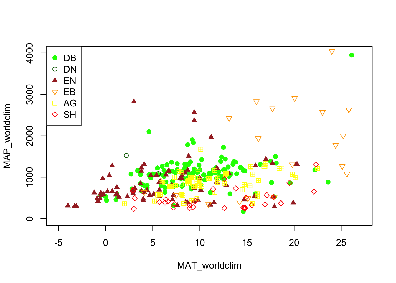
4.7.2 Filtering using attributes
Alternatively, we may want to only include Phenocams with certain attributes in
our datasets. For example, we may be interested only in sites with a co-located
flux tower. For this, we’d want to filter for those with a flux tower using the
flux_sitenames attribute in the metadata.
# store sites with flux_data available and the FLUX site name is specified
phenofluxsites <- phenos[flux_data==TRUE&!is.na(flux_sitenames)&flux_sitenames!='',
                         .(PhenoCam=site, Flux=flux_sitenames)] # return as table
#and specify which variables to retain

phenofluxsites <- phenofluxsites[Flux!='']

# see the first few rows
head(phenofluxsites)
## PhenoCam Flux
## 1: alligatorriver US-NC4
## 2: arsbrooks10 US-Br1: Brooks Field Site 10- Ames
## 3: arsbrooks11 US-Br3: Brooks Field Site 11- Ames
## 4: arscolesnorth LTAR
## 5: arscolessouth LTAR
## 6: arsgreatbasinltar098 US-RwsWe could further identify which of those Phenocams with a flux tower and in
deciduous broadleaf forests (primary_veg_type=='DB').
#list deciduous broadleaf sites with flux tower
DB.flux <- phenos[flux_data==TRUE&primary_veg_type=='DB',
                  site]  # return just the site names as a list

# see the first few rows
head(DB.flux)
## [1] "alligatorriver" "bartlett" "bartlettir" "bbc1"
## [5] "bbc2" "bbc3"4.8 Download midday images
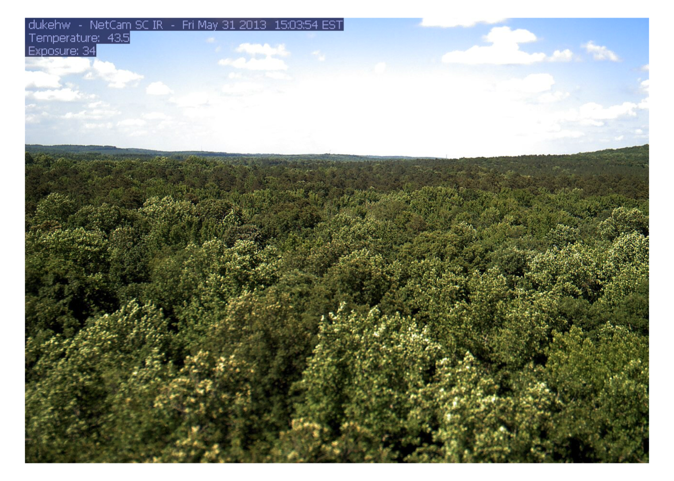
While PhenoCam sites may have many images in a given day, many simple analyses can use just the midday image when the sun is most directly overhead the canopy. Therefore, extracting a list of midday images (only one image a day) can be useful.
# obtaining midday_images for dukehw
duke_middays <- get_midday_list('dukehw')

# see the first few rows
head(duke_middays)
## [1] "http://phenocam.sr.unh.edu/data/archive/dukehw/2013/05/dukehw_2013_05_31_150331.jpg"
## [2] "http://phenocam.sr.unh.edu/data/archive/dukehw/2013/06/dukehw_2013_06_01_120111.jpg"
## [3] "http://phenocam.sr.unh.edu/data/archive/dukehw/2013/06/dukehw_2013_06_02_120109.jpg"
## [4] "http://phenocam.sr.unh.edu/data/archive/dukehw/2013/06/dukehw_2013_06_03_120110.jpg"
## [5] "http://phenocam.sr.unh.edu/data/archive/dukehw/2013/06/dukehw_2013_06_04_120119.jpg"
## [6] "http://phenocam.sr.unh.edu/data/archive/dukehw/2013/06/dukehw_2013_06_05_120110.jpg"Now we have a list of all the midday images from this Phenocam. Let’s download them and plot
# download a file
destfile <- tempfile(fileext = '.jpg')

# download only the first available file
# modify the `[1]` to download other images
download.file(duke_middays[1], destfile = destfile, mode = 'wb')

# plot the image
img <- try(readJPEG(destfile))
if(class(img)!='try-error'){
  par(mar= c(0,0,0,0))
  plot(0:1,0:1, type='n', axes= FALSE, xlab= '', ylab = '')
  rasterImage(img, 0, 0, 1, 1)
}
4.8.1 Download midday images for a given time range
Now we can access all the midday images and download them one at a time. However, we frequently want all the images within a specific time range of interest. We’ll learn how to do that next.
# open a temporary directory
tmp_dir <- tempdir()

# download a subset. Example dukehw 2017
download_midday_images(site = 'dukehw', # which site
                       y = 2017, # which year(s)
                       months = 1:12, # which month(s)
                       days = 15, # which days on month(s)
                       download_dir = tmp_dir) # where on your computer
##
|
| | 0%
|
|====== | 8%
|
|============ | 17%
|
|================== | 25%
|
|======================= | 33%
|
|============================= | 42%
|
|=================================== | 50%
|
|========================================= | 58%
|
|=============================================== | 67%
|
|==================================================== | 75%
|
|========================================================== | 83%
|
|================================================================ | 92%
|
|======================================================================| 100%## [1] "/var/folders/5n/vxrdb72140b43_jhsmhfy514pqgq1n/T//RtmpQu9McA"# list of downloaded files
duke_middays_path <- dir(tmp_dir, pattern = 'dukehw*', full.names = TRUE)
head(duke_middays_path)## [1] "/var/folders/5n/vxrdb72140b43_jhsmhfy514pqgq1n/T//RtmpQu9McA/dukehw_2017_01_15_120109.jpg"
## [2] "/var/folders/5n/vxrdb72140b43_jhsmhfy514pqgq1n/T//RtmpQu9McA/dukehw_2017_02_15_120108.jpg"
## [3] "/var/folders/5n/vxrdb72140b43_jhsmhfy514pqgq1n/T//RtmpQu9McA/dukehw_2017_03_15_120151.jpg"
## [4] "/var/folders/5n/vxrdb72140b43_jhsmhfy514pqgq1n/T//RtmpQu9McA/dukehw_2017_04_15_120110.jpg"
## [5] "/var/folders/5n/vxrdb72140b43_jhsmhfy514pqgq1n/T//RtmpQu9McA/dukehw_2017_05_15_120108.jpg"
## [6] "/var/folders/5n/vxrdb72140b43_jhsmhfy514pqgq1n/T//RtmpQu9McA/dukehw_2017_06_15_120120.jpg"We can demonstrate the seasonality of Duke forest observed from the camera. (Note this code may take a while to run through the loop).
n <- length(duke_middays_path)
par(mar= c(0,0,0,0), mfrow=c(4,3), oma=c(0,0,3,0))

for(i in 1:n){
  img <- readJPEG(duke_middays_path[i])
  plot(0:1,0:1, type='n', axes= FALSE, xlab= '', ylab = '')
  rasterImage(img, 0, 0, 1, 1)
  mtext(month.name[i], line = -2)
}
mtext('Seasonal variation of forest at Duke Hardwood Forest', font = 2, outer = TRUE)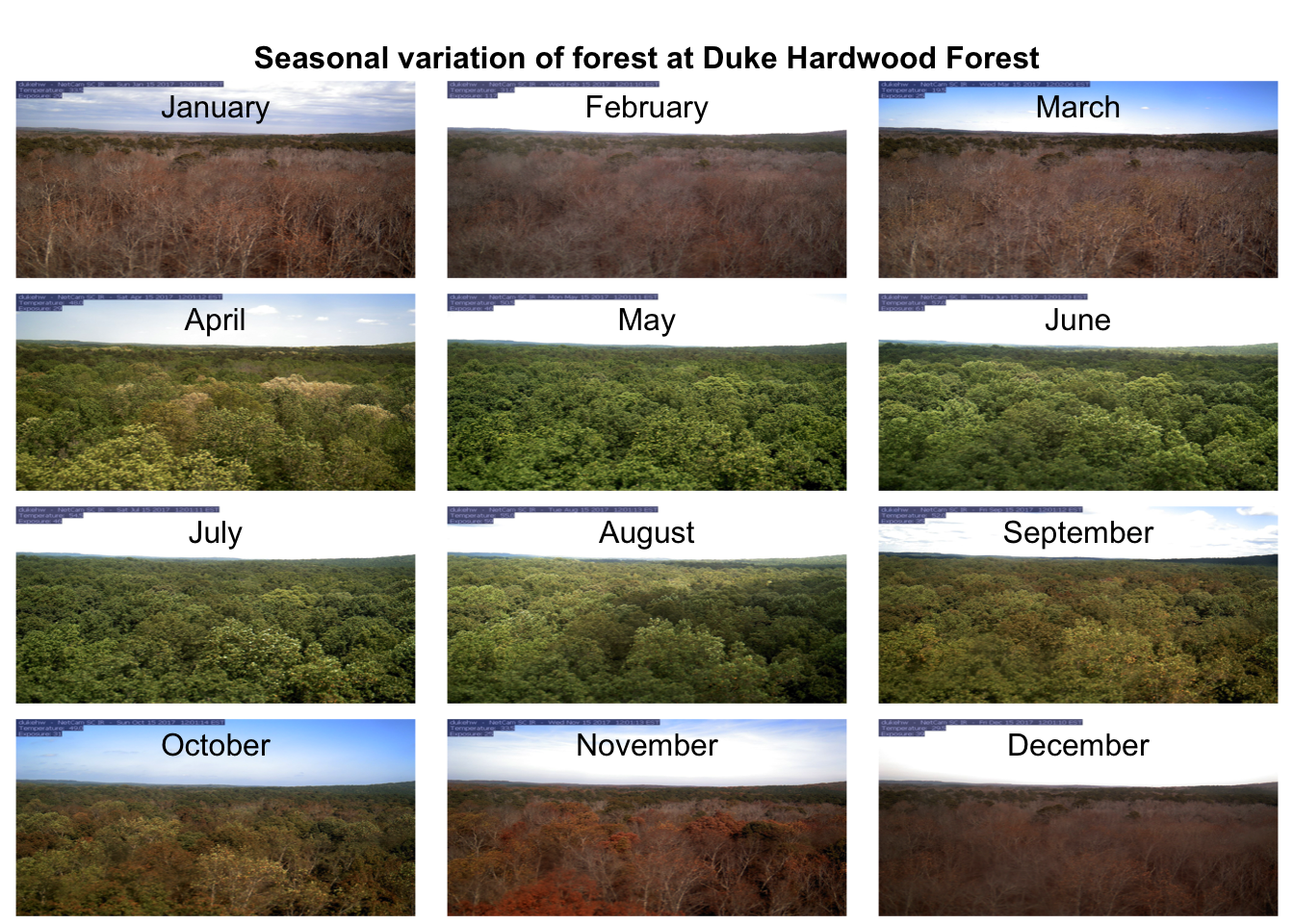
The goal of this section was to show how to download a limited number of midday images from the PhenoCam server. However, more extensive datasets should be downloaded from the PhenoCam .
The phenocamapi R package is developed and maintained by Bijan Seyednarollah. The most recent release is available from https://github.com/bnasr/phenocamapi.
4.9 Detecting Foggy Images using the ‘hazer’ R Package
4.9.0.1 Read & Plot an Image
We will use several packages in this tutorial. All are available from CRAN.
## Warning: package 'dplyr' was built under R version 3.6.2##
## Attaching package: 'dplyr'## The following objects are masked from 'package:data.table':
##
## between, first, last## The following objects are masked from 'package:stats':
##
## filter, lag## The following objects are masked from 'package:base':
##
## intersect, setdiff, setequal, unionBefore we start the image processing steps, let’s read in and plot an image. This image is an example image that comes with the hazer package.
# read the path to the example image
jpeg_file <- system.file(package = 'hazer', 'pointreyes.jpg')

# read the image as an array
rgb_array <- jpeg::readJPEG(jpeg_file)

# plot the RGB array on the active device panel


# first set the margin in this order:(bottom, left, top, right)
par(mar=c(0,0,3,0))
plotRGBArray(rgb_array, bty = 'n', main = 'Point Reyes National Seashore')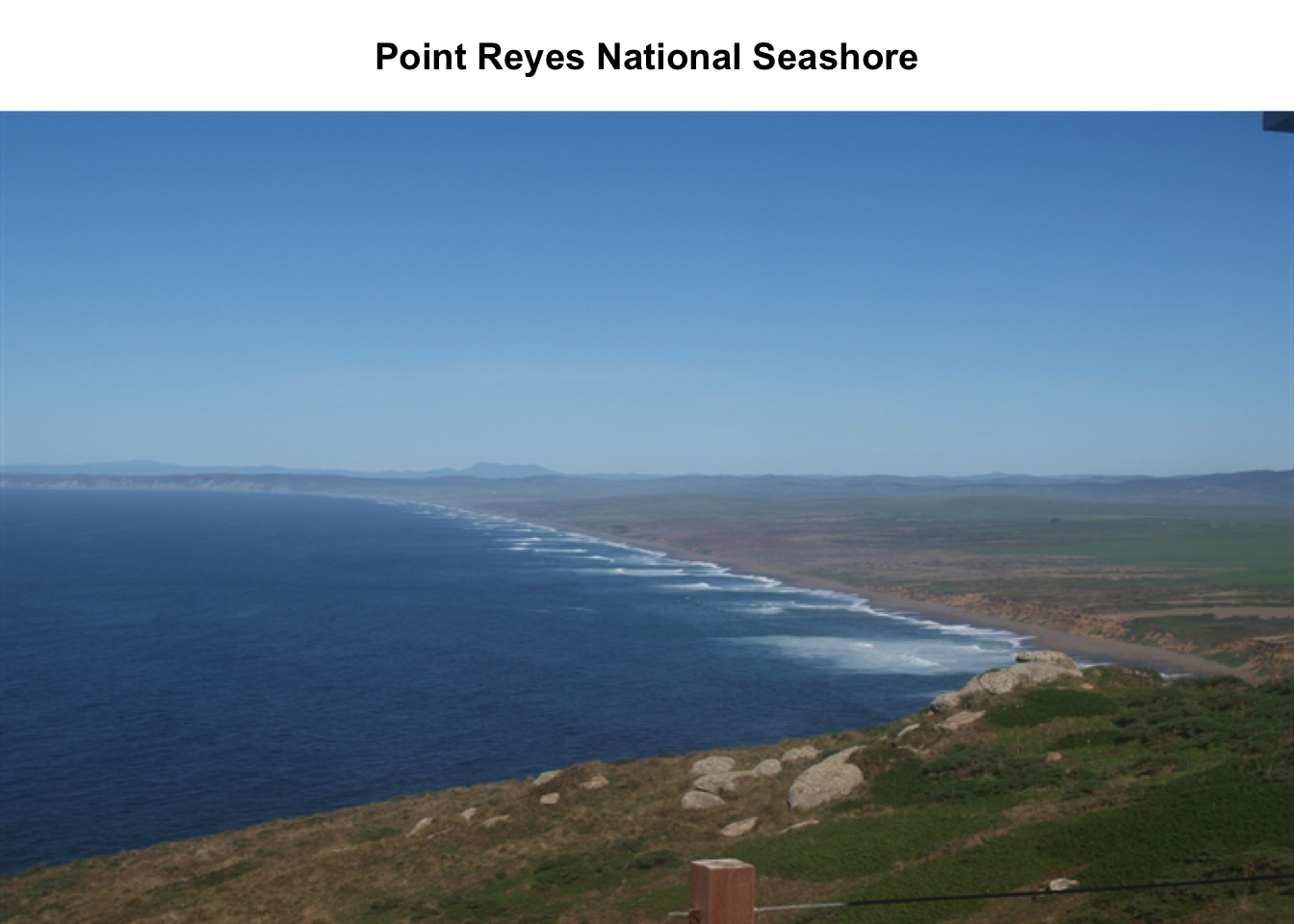
When we work with images, all data we work with is generally on the scale of each individual pixel in the image. Therefore, for large images we will be working with large matrices that hold the value for each pixel. Keep this in mind before opening some of the matrices we’ll be creating this tutorial as it can take a while for them to load.
4.9.0.2 Histogram of RGB channels
A histogram of the colors can be useful to understanding what our image is made
up of. Using the density() function from the base stats package, we can extract
density distribution of each color channel.
# color channels can be extracted from the matrix
red_vector <- rgb_array[,,1]
green_vector <- rgb_array[,,2]
blue_vector <- rgb_array[,,3]

# plotting
par(mar=c(5,4,4,2))
plot(density(red_vector), col = 'red', lwd = 2,
     main = 'Density function of the RGB channels', ylim = c(0,5))
lines(density(green_vector), col = 'green', lwd = 2)
lines(density(blue_vector), col = 'blue', lwd = 2)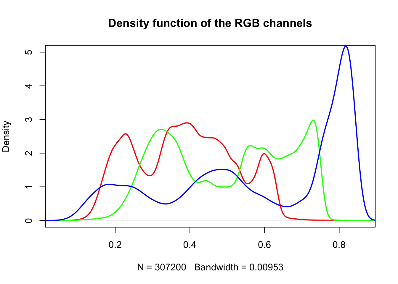
In hazer we can also extract three basic elements of an RGB image :
- Brightness
- Darkness
- Contrast
4.9.0.3 Brightness
The brightness matrix comes from the maximum value of the R, G, or B channel. We
can extract and show the brightness matrix using the getBrightness() function.
# extracting the brightness matrix
brightness_mat <- getBrightness(rgb_array)

# unlike the RGB array which has 3 dimensions, the brightness matrix has only two
# dimensions and can be shown as a grayscale image,
# we can do this using the same plotRGBArray function
par(mar=c(0,0,3,0))
plotRGBArray(brightness_mat, bty = 'n', main = 'Brightness matrix')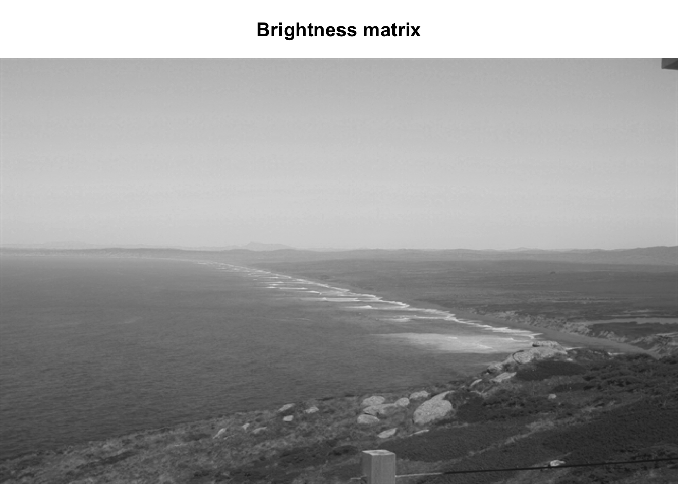
Here the grayscale is used to show the value of each pixel’s maximum brightness of the R, G or B color channel.
To extract a single brightness value for the image, depending on our needs we can perform some statistics or we can just use the mean of this matrix.
##         0%        25%        50%        75%       100%
## 0.09019608 0.43529412 0.62745098 0.80000000 0.91764706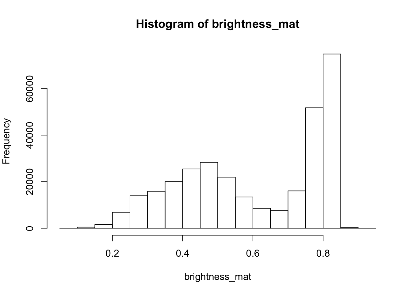
Question for the class: Why are we getting so many images up in the high range of the brightness? Where does this correlate to on the RGB image?
4.9.0.4 Darkness
Darkness is determined by the minimum of the R, G or B color channel. In the
Similarly, we can extract and show the darkness matrix using the getDarkness() function.
# extracting the darkness matrix
darkness_mat <- getDarkness(rgb_array)

# the darkness matrix has also two dimensions and can be shown as a grayscale image
par(mar=c(0,0,3,0))
plotRGBArray(darkness_mat, bty = 'n', main = 'Darkness matrix')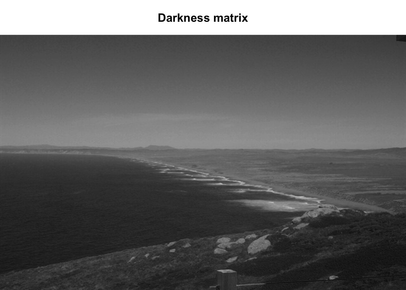
##         0%        25%        50%        75%       100%
## 0.03529412 0.23137255 0.36470588 0.47843137 0.83529412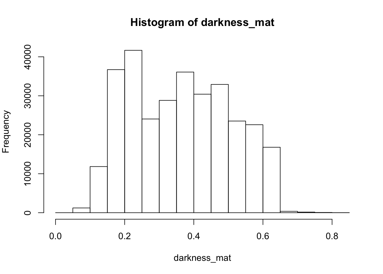
4.9.0.5 Contrast
The contrast of an image is the difference between the darkness and brightness of the image. The contrast matrix is calculated by difference between the darkness and brightness matrices.
The contrast of the image can quickly be extracted using the getContrast() function.
# extracting the contrast matrix
contrast_mat <- getContrast(rgb_array)

# the contrast matrix has also 2D and can be shown as a grayscale image
par(mar=c(0,0,3,0))
plotRGBArray(contrast_mat, bty = 'n', main = 'Contrast matrix')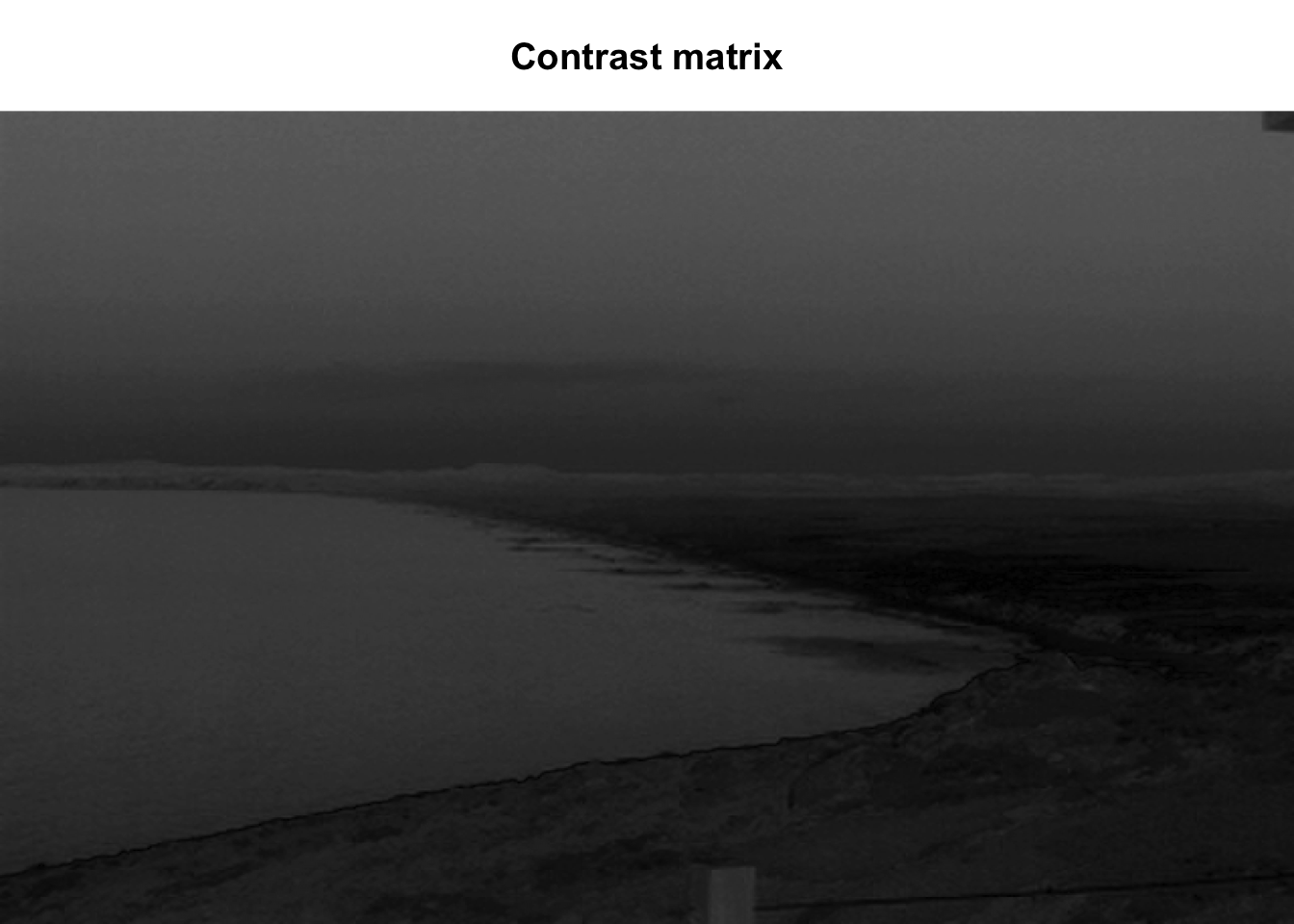
##        0%       25%       50%       75%      100%
## 0.0000000 0.1450980 0.2470588 0.3333333 0.4509804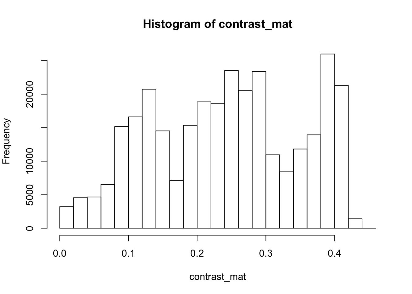
4.9.0.6 Image fogginess & haziness
Haziness of an image can be estimated using the getHazeFactor() function. This
function is based on the method described in
Mao et al. (2014).
The technique was originally developed to for “detecting foggy images and
estimating the haze degree factor” for a wide range of outdoor conditions.
The function returns a vector of two numeric values:
- haze as the haze degree and
- A0 as the global atmospheric light, as it is explained in the original paper.
The PhenoCam standards classify any image with the haze degree greater than 0.4 as a significantly foggy image.
## $haze
## [1] 0.2251633
##
## $A0
## [1] 0.7105258
Here we have the haze values for our image. Note that the values might be slightly different due to rounding errors on different platforms.
4.9.0.7 Process sets of images
We can use for loops or the lapply functions to extract the haze values for
a stack of images.
You can download the related datasets from here (direct download). Download and extract the zip file to be used as input data for the following step.
#pointreyes_url <- 'http://bit.ly/2F8w2Ia'

# set up the input image directory
data_dir <- 'data/'
#dir.create(data_dir, showWarnings = F)

#pointreyes_zip <- paste0(data_dir, 'pointreyes.zip')
pointreyes_dir <- paste0(data_dir, 'pointreyes')

#download zip file
#download.file(pointreyes_url, destfile = pointreyes_zip)
#unzip(pointreyes_zip, exdir = data_dir)

# get a list of all .jpg files in the directory
pointreyes_images <- dir(path = 'data/pointreyes',
                         pattern = '*.jpg',
                         ignore.case = TRUE,
                         full.names = TRUE)
Now we can use a for loop to process all of the images to get the haze and A0 values.
# number of images
n <- length(pointreyes_images)

# create an empty matrix to fill with haze and A0 values
haze_mat <- data.frame()

# the process takes a bit, a progress bar lets us know it is working.
pb <- txtProgressBar(0, n, style = 3)
##
|
| | 0%for(i in 1:n) {
image_path <- pointreyes_images[i]
img <- jpeg::readJPEG(image_path)
hz <- getHazeFactor(img)
haze_mat <- rbind(haze_mat,
data.frame(file = as.character(image_path),
haze = hz[1],
A0 = hz[2]))
setTxtProgressBar(pb, i)
}##
|
|= | 1%
|
|== | 3%
|
|=== | 4%
|
|==== | 6%
|
|===== | 7%
|
|====== | 8%
|
|======= | 10%
|
|======== | 11%
|
|========= | 13%
|
|========== | 14%
|
|=========== | 15%
|
|============ | 17%
|
|============= | 18%
|
|============== | 20%
|
|=============== | 21%
|
|================ | 23%
|
|================= | 24%
|
|================== | 25%
|
|=================== | 27%
|
|==================== | 28%
|
|===================== | 30%
|
|====================== | 31%
|
|======================= | 32%
|
|======================== | 34%
|
|========================= | 35%
|
|========================== | 37%
|
|=========================== | 38%
|
|============================ | 39%
|
|============================= | 41%
|
|============================== | 42%
|
|=============================== | 44%
|
|================================ | 45%
|
|================================= | 46%
|
|================================== | 48%
|
|=================================== | 49%
|
|=================================== | 51%
|
|==================================== | 52%
|
|===================================== | 54%
|
|====================================== | 55%
|
|======================================= | 56%
|
|======================================== | 58%
|
|========================================= | 59%
|
|========================================== | 61%
|
|=========================================== | 62%
|
|============================================ | 63%
|
|============================================= | 65%
|
|============================================== | 66%
|
|=============================================== | 68%
|
|================================================ | 69%
|
|================================================= | 70%
|
|================================================== | 72%
|
|=================================================== | 73%
|
|==================================================== | 75%
|
|===================================================== | 76%
|
|====================================================== | 77%
|
|======================================================= | 79%
|
|======================================================== | 80%
|
|========================================================= | 82%
|
|========================================================== | 83%
|
|=========================================================== | 85%
|
|============================================================ | 86%
|
|============================================================= | 87%
|
|============================================================== | 89%
|
|=============================================================== | 90%
|
|================================================================ | 92%
|
|================================================================= | 93%
|
|================================================================== | 94%
|
|=================================================================== | 96%
|
|==================================================================== | 97%
|
|===================================================================== | 99%
|
|======================================================================| 100%Now we have a matrix with haze and A0 values for all our images. Let’s compare top three images with low and high haze values.
top10_high_haze <- haze_mat %>%
  dplyr::arrange(desc(haze)) %>%
  slice(1:3)
top10_low_haze <-  haze_mat %>%
  arrange(haze)%>%
  slice(1:3)


par(mar= c(0,0,0,0), mfrow=c(3,2), oma=c(0,0,3,0))

for(i in 1:3){
  img <- readJPEG(as.character(top10_low_haze$file[i]))
  plot.new()
  rasterImage(img, par()$usr[1], par()$usr[3], par()$usr[2], par()$usr[4])

  img <- readJPEG(as.character(top10_high_haze$file[i]))
  plot.new()
  rasterImage(img, par()$usr[1], par()$usr[3], par()$usr[2], par()$usr[4])

}
mtext('Top images with low (left) and high (right) haze values at Point Reyes', font = 2, outer = TRUE)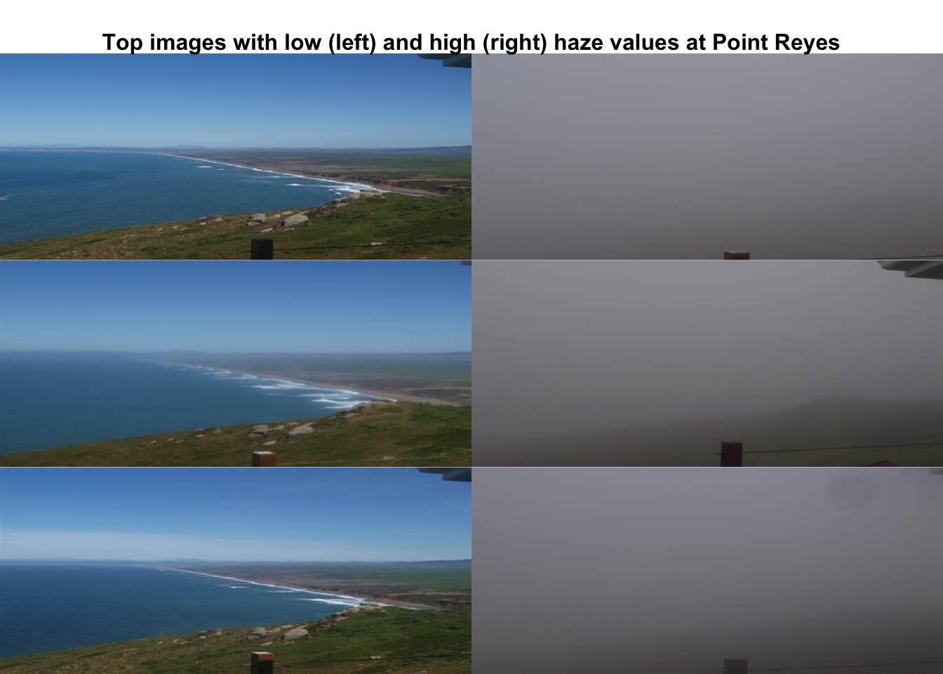
Let’s classify those into hazy and non-hazy as per the PhenoCam standard of 0.4.
# classify image as hazy: T/F
haze_mat=haze_mat%>%
  mutate(haze_mat, foggy=ifelse(haze>.4, TRUE, FALSE))

head(haze_mat)
## file haze A0 foggy
## 1 data/pointreyes/pointreyes_2017_01_01_120056.jpg 0.2249810 0.6970257 FALSE
## 2 data/pointreyes/pointreyes_2017_01_06_120210.jpg 0.2339372 0.6826148 FALSE
## 3 data/pointreyes/pointreyes_2017_01_16_120105.jpg 0.2312940 0.7009978 FALSE
## 4 data/pointreyes/pointreyes_2017_01_21_120105.jpg 0.4536108 0.6209055 TRUE
## 5 data/pointreyes/pointreyes_2017_01_26_120106.jpg 0.2297961 0.6813884 FALSE
## 6 data/pointreyes/pointreyes_2017_01_31_120125.jpg 0.4206842 0.6315728 TRUENow we can save all the foggy images to a new folder that will retain the foggy images but keep them separate from the non-foggy ones that we want to analyze.
# identify directory to move the foggy images to
foggy_dir <- paste0(pointreyes_dir, 'foggy')
clear_dir <- paste0(pointreyes_dir, 'clear')

# if a new directory, create new directory at this file path
dir.create(foggy_dir,  showWarnings = FALSE)
dir.create(clear_dir,  showWarnings = FALSE)

# copy the files to the new directories
#file.copy(haze_mat[foggy==TRUE,file], to = foggy_dir)

#file.copy(haze_mat[foggy==FALSE,file], to = clear_dir)
Now that we have our images separated, we can get the full list of haze values only for those images that are not classified as “foggy”.
# this is an alternative approach instead of a for loop

# loading all the images as a list of arrays
pointreyes_clear_images <- dir(path = clear_dir,
                               pattern = '*.jpg',
                               ignore.case = TRUE,
                               full.names = TRUE)

img_list <- lapply(pointreyes_clear_images, FUN = jpeg::readJPEG)

# getting the haze value for the list
# patience - this takes a bit of time
haze_list <- t(sapply(img_list, FUN = getHazeFactor))

# view first few entries
head(haze_list)
## haze A0
## [1,] 0.224981 0.6970257
## [2,] 0.2339372 0.6826148
## [3,] 0.231294 0.7009978
## [4,] 0.2297961 0.6813884
## [5,] 0.2152078 0.6949932
## [6,] 0.345584 0.6789334We can then use these values for further analyses and data correction.
The hazer R package is developed and maintained by Bijan Seyednarollah. The most recent release is available from https://github.com/bnasr/hazer.
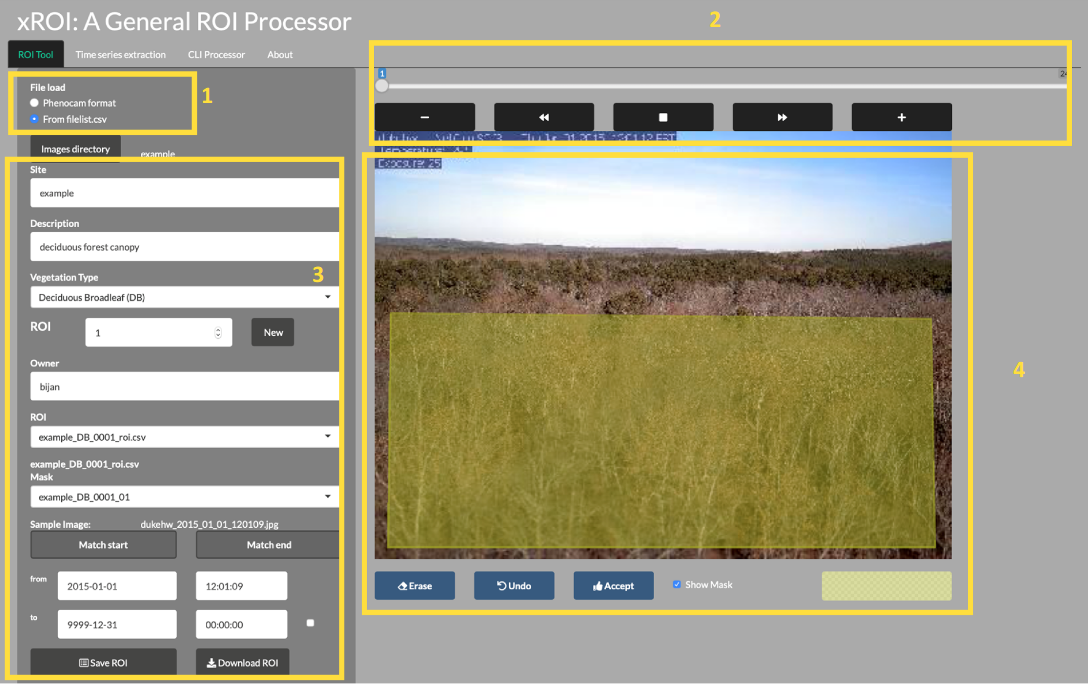
4.10 Extracting Timeseries from Images using the xROI R Package
In this section, we’ll learn how to use an interactive open-source toolkit, the xROI R package that facilitates the process of time series extraction and improves the quality of the final data. The xROI package provides a responsive environment for scientists to interactively:
- delineate regions of interest (ROIs),
- handle field of view (FOV) shifts, and
- extract and export time series data characterizing color-based metrics.
Using the xROI R package, the user can detect FOV shifts with minimal difficulty. The software gives user the opportunity to re-adjust mask files or redraw new ones every time an FOV shift occurs.
4.10.1 xROI Design
The R language and Shiny package were used as the main development tool for xROI,
while Markdown, HTML, CSS and JavaScript languages were used to improve the
interactivity. While Shiny apps are primarily used for web-based applications to
be used online, the package authors used Shiny for its graphical user interface
capabilities. In other words, both the User Interface (UI) and server modules are run
locally from the same machine and hence no internet connection is required (after
installation). The xROI’s UI element presents a side-panel for data entry and
three main tab-pages, each responsible for a specific task. The server-side
element consists of R and bash scripts. Image processing and geospatial features
were performed using the Geospatial Data Abstraction Library (GDAL) and the
rgdal and raster R packages.
4.10.2 Install xROI
The xROI R package has been published on The Comprehensive R Archive Network (CRAN). The latest tested xROI package can be installed from the CRAN packages repository by running the following command in an R environment.
Alternatively, the latest beta release of xROI can be directly downloaded and installed from the development GitHub repository.
# install devtools first
utils::install.packages('devtools', repos = "http://cran.us.r-project.org" )

# use devtools to install from GitHub
devtools::install_github("bnasr/xROI")
xROI depends on many R packages including: raster, rgdal, sp, jpeg,
tiff, shiny, shinyjs, shinyBS, shinyAce, shinyTime, shinyFiles,
shinydashboard, shinythemes, colourpicker, rjson, stringr, data.table,
lubridate, plotly, moments, and RCurl. All the required libraries and
packages will be automatically installed with installation of xROI. The package
offers a fully interactive high-level interface as well as a set of low-level
functions for ROI processing.
4.10.3 Launch xROI
A comprehensive user manual for low-level image processing using xROI is available from CRAN xROI.pdf. While the user manual includes a set of examples for each function; here we will learn to use the graphical interactive mode.
Calling the Launch() function, as we’ll do below, opens up the interactive
mode in your operating system’s default web browser. The landing page offers an
example dataset to explore different modules or upload a new dataset of images.
You can launch the interactive mode can be launched from an interactive R environment.
Or from the command line (e.g. bash in Linux, Terminal in macOS and Command Prompt in Windows machines) where an R engine is already installed.
4.10.4 End xROI
When you are done with the xROI interface you can close the tab in your browser and end the session in R by using one of the following options
In RStudio: Press the
4.10.5 Use xROI
To get some hands-on experience with xROI, we can analyze images from the
dukehw
of the PhenoCam network.
You can download the data set from this link (direct download).
Follow the steps below:
First,save and extract (unzip) the file on your computer.
Second, open the data set in xROI by setting the file path to your data
# launch data in ROI
# first edit the path below to the dowloaded directory you just extracted
xROI::Launch('/path/to/extracted/directory')

# alternatively, you can run without specifying a path and use the interface to browse
Now, draw an ROI and the metadata.
Then, save the metadata and explore its content.
Now we can explore if there is any FOV shift in the dataset using the CLI processer tab.
Finally, we can go to the Time series extraction tab. Extract the time-series. Save the output and explore the dataset in R.
4.11 Documentation and Citation
More documentation about xROI can be found from: Seyednarollah, et al. 2019.
 >xROI published in ISPRS Journal of Photogrammetry and Remote Sensing, 2019
4.11.1 Challenge: Use xROI
Let’s use xROI on a little more challenging site with field of view shifts.
Download and extract the data set from this link (direct download, 218 MB) and follow the above steps to extract the time-series.
The xROI R package is developed and maintained by Bijan Seyednarollah. The most recent release is available from https://github.com/bnasr/xROI.
4.12 Hands on: Digital Repeat Photography Computational
First let’s load some packages:
##
## Attaching package: 'jsonlite'
## The following objects are masked from 'package:rjson':
##
## fromJSON, toJSON## Loading required package: ggplot2##
## Attaching package: 'plotly'## The following object is masked from 'package:ggplot2':
##
## last_plot## The following object is masked from 'package:stats':
##
## filter## The following object is masked from 'package:graphics':
##
## layoutAs a refresher, there are two main ways to pull in PhenoCam data. First, directly via the API:
c      = jsonlite::fromJSON('https://phenocam.sr.unh.edu/api/cameras/?format=json&limit=2000')
c = c$results
c_m=c$sitemetadata
c$sitemetadata=NULL
cams_=cbind(c, c_m)
cams_[is.na(cams_)] = 'N'
cams_[, 2:4] <- sapply(cams_[, 2:4], as.numeric) #changing lat/lon/elev from string values into numeric
## Warning in lapply(X = X, FUN = FUN, ...): NAs introduced by coercion
## Warning in lapply(X = X, FUN = FUN, ...): NAs introduced by coercion
## Warning in lapply(X = X, FUN = FUN, ...): NAs introduced by coercion## Sitename Lat Lon Elev active utc_offset date_first
## 1 aafcottawacfiaf14e 45.29210 -75.76640 90 TRUE -5 2020-04-27
## 2 aafcottawacfiaf14w 45.29210 -75.76640 90 TRUE -5 2020-05-01
## 3 acadia 44.37694 -68.26083 158 TRUE -5 2007-03-15
## 4 aguatibiaeast 33.62200 -116.86700 1086 FALSE -8 2007-08-16
## 5 aguatibianorth 33.60222 -117.34368 1090 FALSE -8 2003-10-01
## 6 ahwahnee 37.74670 -119.58160 1199 TRUE -8 2008-08-28
## date_last infrared contact1
## 1 2021-02-08 N Elizabeth Pattey <elizabeth DOT pattey AT canada DOT ca>
## 2 2021-02-08 N Elizabeth Pattey <elizabeth DOT pattey AT canada DOT ca>
## 3 2021-02-11 N Dee Morse <dee_morse AT nps DOT gov>
## 4 2019-01-25 N Ann E Mebane <amebane AT fs DOT fed DOT us>
## 5 2006-10-25 N
## 6 2021-02-11 N Dee Morse <dee_morse AT nps DOT gov>
## contact2
## 1 Luc Pelletier <luc DOT pelletier3 AT canada DOT ca>
## 2 Luc Pelletier <luc DOT pelletier3 AT canada DOT ca>
## 3 John Gross <John_Gross AT nps DOT gov>
## 4 Kristi Savig <KSavig AT air-resource DOT com>
## 5
## 6 John Gross <John_Gross AT nps DOT gov>
## site_description site_type
## 1 AAFC Site - Ottawa (On) - CFIA - Field F14 -East Flux Tower II
## 2 AAFC Site - Ottawa (On) - CFIA - Field F14 -West Flux Tower II
## 3 Acadia National Park, McFarland Hill, near Bar Harbor, Maine III
## 4 Agua Tibia Wilderness, California III
## 5 Agua Tibia Wilderness, California III
## 6 Ahwahnee Meadow, Yosemite National Park, California III
## group camera_description camera_orientation flux_data
## 1 N Campbell Scientific CCFC NE TRUE
## 2 N Campbell Scientific CCFC WNW TRUE
## 3 National Park Service unknown NE FALSE
## 4 USFS unknown SW FALSE
## 5 USFS unknown NE FALSE
## 6 National Park Service unknown E FALSE
## flux_networks flux_sitenames
## 1 NULL N
## 2 OTHER, , Other/Unaffiliated N
## 3 NULL
## 4 NULL
## 5 NULL
## 6 NULL
## dominant_species primary_veg_type
## 1 Zea mays, Triticum aestivum, Brassica napus, Glycine max AG
## 2 Zea mays, Triticum aestivum, Brassica napus, Glycine max AG
## 3 DB
## 4 SH
## 5 SH
## 6 EN
## secondary_veg_type site_meteorology MAT_site MAP_site MAT_daymet MAP_daymet
## 1 AG TRUE 6.4 943 6.3 952
## 2 AG TRUE 6.4 943 6.3 952
## 3 EN FALSE N N 7.05 1439
## 4 FALSE N N 15.75 483
## 5 FALSE N N 16 489
## 6 GR FALSE N N 12.25 871
## MAT_worldclim MAP_worldclim koeppen_geiger ecoregion landcover_igbp
## 1 6 863 Dfb 8 12
## 2 6 863 Dfb 8 12
## 3 6.5 1303 Dfb 8 5
## 4 14.9 504 Csa 11 7
## 5 13.8 729 Csa 11 7
## 6 11.8 886 Csb 6 8
## site_acknowledgements
## 1 Camera funded by Agriculture and Agri-Food Canada (AAFC) Project J-001735 - Commercial inhibitors’ impact on crop productivity and emissions of nitrous oxide led by Dr. Elizabeth Pattey; Support provided by Drs, Luc Pelletier and Elizabeth Pattey, Micrometeorologiccal Laboratory of AAFC - Ottawa Research and Development Centre.
## 2 Cameras funded by Agriculture and Agri-Food Canada (AAFC) Project J-001735 - Commercial inhibitors’ impact on crop productivity and emissions of nitrous oxide led by Dr. Elizabeth Pattey; Support provided by Drs, Luc Pelletier and Elizabeth Pattey, Micrometeorologiccal Laboratory of AAFC - Ottawa Research and Development Centre.
## 3 Camera images from Acadia National Park are provided courtesy of the National Park Service Air Resources Program.
## 4 Camera images from Agua Tibia Wilderness are provided courtesy of the USDA Forest Service Air Resources Management Program.
## 5 Camera images from Agua Tibia Wilderness are provided courtesy of the USDA Forest Service Air Resources Management Program.
## 6 Camera images from Yosemite National Park are provided courtesy of the National Park Service Air Resources Program.
## modified
## 1 2020-05-04T10:46:30.065790-04:00
## 2 2020-05-04T10:46:32.523976-04:00
## 3 2016-11-01T15:42:15.016778-04:00
## 4 2016-11-01T15:42:15.086984-04:00
## 5 2016-11-01T15:42:15.095277-04:00
## 6 2016-11-01T15:42:15.111916-04:00And second, via the phenocamapi package:
##                  site      lat        lon elev active utc_offset date_first
## 1: aafcottawacfiaf14e 45.29210  -75.76640   90   TRUE         -5 2020-04-27
## 2: aafcottawacfiaf14w 45.29210  -75.76640   90   TRUE         -5 2020-05-01
## 3:             acadia 44.37694  -68.26083  158   TRUE         -5 2007-03-15
## 4:      aguatibiaeast 33.62200 -116.86700 1086  FALSE         -8 2007-08-16
## 5:     aguatibianorth 33.60222 -117.34368 1090  FALSE         -8 2003-10-01
## 6:           ahwahnee 37.74670 -119.58160 1199   TRUE         -8 2008-08-28
##     date_last infrared                                      contact1
## 1: 2021-02-08        N Elizabeth Pattey <elizabeth.pattey@canada.ca>
## 2: 2021-02-08        N Elizabeth Pattey <elizabeth.pattey@canada.ca>
## 3: 2021-02-11        N                 Dee Morse <dee_morse@nps.gov>
## 4: 2019-01-25        N              Ann E Mebane <amebane@fs.fed.us>
## 5: 2006-10-25        N
## 6: 2021-02-11        N                 Dee Morse <dee_morse@nps.gov>
##                                    contact2
## 1: Luc Pelletier <luc.pelletier3@canada.ca>
## 2: Luc Pelletier <luc.pelletier3@canada.ca>
## 3:          John Gross <John_Gross@nps.gov>
## 4:   Kristi Savig <KSavig@air-resource.com>
## 5:
## 6:          John Gross <John_Gross@nps.gov>
##                                                site_description site_type
## 1:  AAFC Site - Ottawa (On) - CFIA - Field F14 -East Flux Tower        II
## 2:  AAFC Site - Ottawa (On) - CFIA - Field F14 -West Flux Tower        II
## 3: Acadia National Park, McFarland Hill, near Bar Harbor, Maine       III
## 4:                            Agua Tibia Wilderness, California       III
## 5:                            Agua Tibia Wilderness, California       III
## 6:          Ahwahnee Meadow, Yosemite National Park, California       III
##                    group       camera_description camera_orientation flux_data
## 1:                  <NA> Campbell Scientific CCFC                 NE      TRUE
## 2:                  <NA> Campbell Scientific CCFC                WNW      TRUE
## 3: National Park Service                  unknown                 NE     FALSE
## 4:                  USFS                  unknown                 SW     FALSE
## 5:                  USFS                  unknown                 NE     FALSE
## 6: National Park Service                  unknown                  E     FALSE
##    flux_networks flux_sitenames
## 1:     <list[0]>           <NA>
## 2:     <list[1]>           <NA>
## 3:     <list[0]>
## 4:     <list[0]>
## 5:     <list[0]>
## 6:     <list[0]>
##                                            dominant_species primary_veg_type
## 1: Zea mays, Triticum aestivum, Brassica napus, Glycine max               AG
## 2: Zea mays, Triticum aestivum, Brassica napus, Glycine max               AG
## 3:                                                                        DB
## 4:                                                                        SH
## 5:                                                                        SH
## 6:                                                                        EN
##    secondary_veg_type site_meteorology MAT_site MAP_site MAT_daymet MAP_daymet
## 1:                 AG             TRUE      6.4      943       6.30        952
## 2:                 AG             TRUE      6.4      943       6.30        952
## 3:                 EN            FALSE       NA       NA       7.05       1439
## 4:                               FALSE       NA       NA      15.75        483
## 5:                               FALSE       NA       NA      16.00        489
## 6:                 GR            FALSE       NA       NA      12.25        871
##    MAT_worldclim MAP_worldclim koeppen_geiger ecoregion landcover_igbp
## 1:           6.0           863            Dfb         8             12
## 2:           6.0           863            Dfb         8             12
## 3:           6.5          1303            Dfb         8              5
## 4:          14.9           504            Csa        11              7
## 5:          13.8           729            Csa        11              7
## 6:          11.8           886            Csb         6              8
##    dataset_version1
## 1:               NA
## 2:               NA
## 3:               NA
## 4:               NA
## 5:               NA
## 6:               NA
##                                                                                                                                                                                                                                                                                                                          site_acknowledgements
## 1:  Camera funded by Agriculture and Agri-Food Canada (AAFC) Project J-001735 - Commercial inhibitors’ impact on crop productivity and emissions of nitrous oxide led by Dr. Elizabeth Pattey; Support provided by Drs, Luc Pelletier and Elizabeth  Pattey, Micrometeorologiccal Laboratory of AAFC - Ottawa Research and Development Centre.
## 2: Cameras funded by Agriculture and Agri-Food Canada (AAFC) Project J-001735 - Commercial inhibitors’ impact on crop productivity and emissions of nitrous oxide led by Dr. Elizabeth Pattey; Support provided by Drs, Luc Pelletier and Elizabeth  Pattey, Micrometeorologiccal Laboratory of AAFC - Ottawa Research and Development Centre.
## 3:                                                                                                                                                                                                                           Camera images from Acadia National Park are provided courtesy of the National Park Service Air Resources Program.
## 4:                                                                                                                                                                                                                 Camera images from Agua Tibia Wilderness are provided courtesy of the USDA Forest Service Air Resources Management Program.
## 5:                                                                                                                                                                                                                 Camera images from Agua Tibia Wilderness are provided courtesy of the USDA Forest Service Air Resources Management Program.
## 6:                                                                                                                                                                                                                         Camera images from Yosemite National Park are provided courtesy of the National Park Service Air Resources Program.
##                            modified flux_networks_name flux_networks_url
## 1: 2020-05-04T10:46:30.065790-04:00               <NA>              <NA>
## 2: 2020-05-04T10:46:32.523976-04:00              OTHER
## 3: 2016-11-01T15:42:15.016778-04:00               <NA>              <NA>
## 4: 2016-11-01T15:42:15.086984-04:00               <NA>              <NA>
## 5: 2016-11-01T15:42:15.095277-04:00               <NA>              <NA>
## 6: 2016-11-01T15:42:15.111916-04:00               <NA>              <NA>
##    flux_networks_description
## 1:                      <NA>
## 2:        Other/Unaffiliated
## 3:                      <NA>
## 4:                      <NA>
## 5:                      <NA>
## 6:                      <NA>
To familiarize yourself with the phenocam API, let’s explore the structure: https://phenocam.sr.unh.edu/api/
Explore the options for filtering, file type and so forth.
4.12.1 PhenoCam time series
PhenoCam time series are extracted time series data obtained from ROI’s for a given site.
4.12.2 Obtain ROIs
To download the phenological time series from the PhenoCam, we need to know the
site name, vegetation type and ROI ID. This information can be obtained from each
specific PhenoCam page on the
PhenoCam website
or by using the get_rois() function.
# obtaining the list of all the available ROI's on the PhenoCam server
rois <- get_rois()

# view what information is returned
colnames(rois)
## [1] "roi_name" "site" "lat"
## [4] "lon" "roitype" "active"
## [7] "show_link" "show_data_link" "sequence_number"
## [10] "description" "first_date" "last_date"
## [13] "site_years" "missing_data_pct" "roi_page"
## [16] "roi_stats_file" "one_day_summary" "three_day_summary"
## [19] "data_release"## [1] "alligatorriver_DB_1000" "arbutuslake_DB_1000"
## [3] "arbutuslakeinlet_DB_1000" "arbutuslakeinlet_EN_1000"
## [5] "arbutuslakeinlet_EN_2000" "archboldavir_AG_1000"4.12.3 Download time series
The get_pheno_ts() function can download a time series and return the result
as a data.table.
Let’s work with the
Duke Forest Hardwood Stand (dukehw) PhenoCam
and specifically the ROI
DB_1000
we can run the following code.
##          roi_name   site      lat       lon roitype active show_link
## 1: dukehw_DB_1000 dukehw 35.97358 -79.10037      DB   TRUE      TRUE
##    show_data_link sequence_number                                   description
## 1:           TRUE            1000 canopy level DB forest at awesome Duke forest
##    first_date  last_date site_years missing_data_pct
## 1: 2013-06-01 2020-12-24        7.3              3.0
##                                                  roi_page
## 1: https://phenocam.sr.unh.edu/webcam/roi/dukehw/DB_1000/
##                                                                     roi_stats_file
## 1: https://phenocam.sr.unh.edu/data/archive/dukehw/ROI/dukehw_DB_1000_roistats.csv
##                                                                one_day_summary
## 1: https://phenocam.sr.unh.edu/data/archive/dukehw/ROI/dukehw_DB_1000_1day.csv
##                                                              three_day_summary
## 1: https://phenocam.sr.unh.edu/data/archive/dukehw/ROI/dukehw_DB_1000_3day.csv
##    data_release
## 1:           NA
# to obtain the DB 1000 from dukehw
dukehw_DB_1000 <- get_pheno_ts(site = 'dukehw', vegType = 'DB', roiID = 1000, type = '3day')
# what data are available
str(dukehw_DB_1000)## Classes 'data.table' and 'data.frame': 924 obs. of 35 variables:
## $ date : Factor w/ 924 levels "2013-06-01","2013-06-04",..: 1 2 3 4 5 6 7 8 9 10 ...
## $ year : int 2013 2013 2013 2013 2013 2013 2013 2013 2013 2013 ...
## $ doy : int 152 155 158 161 164 167 170 173 176 179 ...
## $ image_count : int 57 76 77 77 77 78 21 0 0 0 ...
## $ midday_filename : Factor w/ 895 levels "dukehw_2013_06_01_120111.jpg",..: 1 2 3 4 5 6 7 895 895 895 ...
## $ midday_r : num 91.3 76.4 60.6 76.5 88.9 ...
## $ midday_g : num 97.9 85 73.2 82.2 95.7 ...
## $ midday_b : num 47.4 33.6 35.6 37.1 51.4 ...
## $ midday_gcc : num 0.414 0.436 0.432 0.42 0.406 ...
## $ midday_rcc : num 0.386 0.392 0.358 0.391 0.377 ...
## $ r_mean : num 87.6 79.9 72.7 80.9 83.8 ...
## $ r_std : num 5.9 6 9.5 8.23 5.89 ...
## $ g_mean : num 92.1 86.9 84 88 89.7 ...
## $ g_std : num 6.34 5.26 7.71 7.77 6.47 ...
## $ b_mean : num 46.1 38 39.6 43.1 46.7 ...
## $ b_std : num 4.48 3.42 5.29 4.73 4.01 ...
## $ gcc_mean : num 0.408 0.425 0.429 0.415 0.407 ...
## $ gcc_std : num 0.00859 0.0089 0.01318 0.01243 0.01072 ...
## $ gcc_50 : num 0.408 0.427 0.431 0.416 0.407 ...
## $ gcc_75 : num 0.414 0.431 0.435 0.424 0.415 ...
## $ gcc_90 : num 0.417 0.434 0.44 0.428 0.421 ...
## $ rcc_mean : num 0.388 0.39 0.37 0.381 0.38 ...
## $ rcc_std : num 0.01176 0.01032 0.01326 0.00881 0.00995 ...
## $ rcc_50 : num 0.387 0.391 0.373 0.383 0.382 ...
## $ rcc_75 : num 0.391 0.396 0.378 0.388 0.385 ...
## $ rcc_90 : num 0.397 0.399 0.382 0.391 0.389 ...
## $ max_solar_elev : num 76 76.3 76.6 76.8 76.9 ...
## $ snow_flag : logi NA NA NA NA NA NA ...
## $ outlierflag_gcc_mean: logi NA NA NA NA NA NA ...
## $ outlierflag_gcc_50 : logi NA NA NA NA NA NA ...
## $ outlierflag_gcc_75 : logi NA NA NA NA NA NA ...
## $ outlierflag_gcc_90 : logi NA NA NA NA NA NA ...
## $ YEAR : int 2013 2013 2013 2013 2013 2013 2013 2013 2013 2013 ...
## $ DOY : int 152 155 158 161 164 167 170 173 176 179 ...
## $ YYYYMMDD : chr "2013-06-01" "2013-06-04" "2013-06-07" "2013-06-10" ...
## - attr(*, ".internal.selfref")=<externalptr>We now have a variety of data related to this ROI from the Hardwood Stand at Duke Forest.
Green Chromatic Coordinate (GCC) is a measure of “greenness” of an area and is
widely used in Phenocam images as an indicator of the green pigment in vegetation.
Let’s use this measure to look at changes in GCC over time at this site. Looking
back at the available data, we have several options for GCC. gcc90 is the 90th
quantile of GCC in the pixels across the ROI (for more details,
PhenoCam v1 description).
We’ll use this as it tracks the upper greenness values while not including many
outliners.
Before we can plot gcc-90 we do need to fix our dates and convert them from
Factors to Date to correctly plot.
# date variable into date format
dukehw_DB_1000[,date:=as.Date(date)]

# plot gcc_90
dukehw_DB_1000[,plot(date, gcc_90, col = 'green', type = 'b')]
## NULL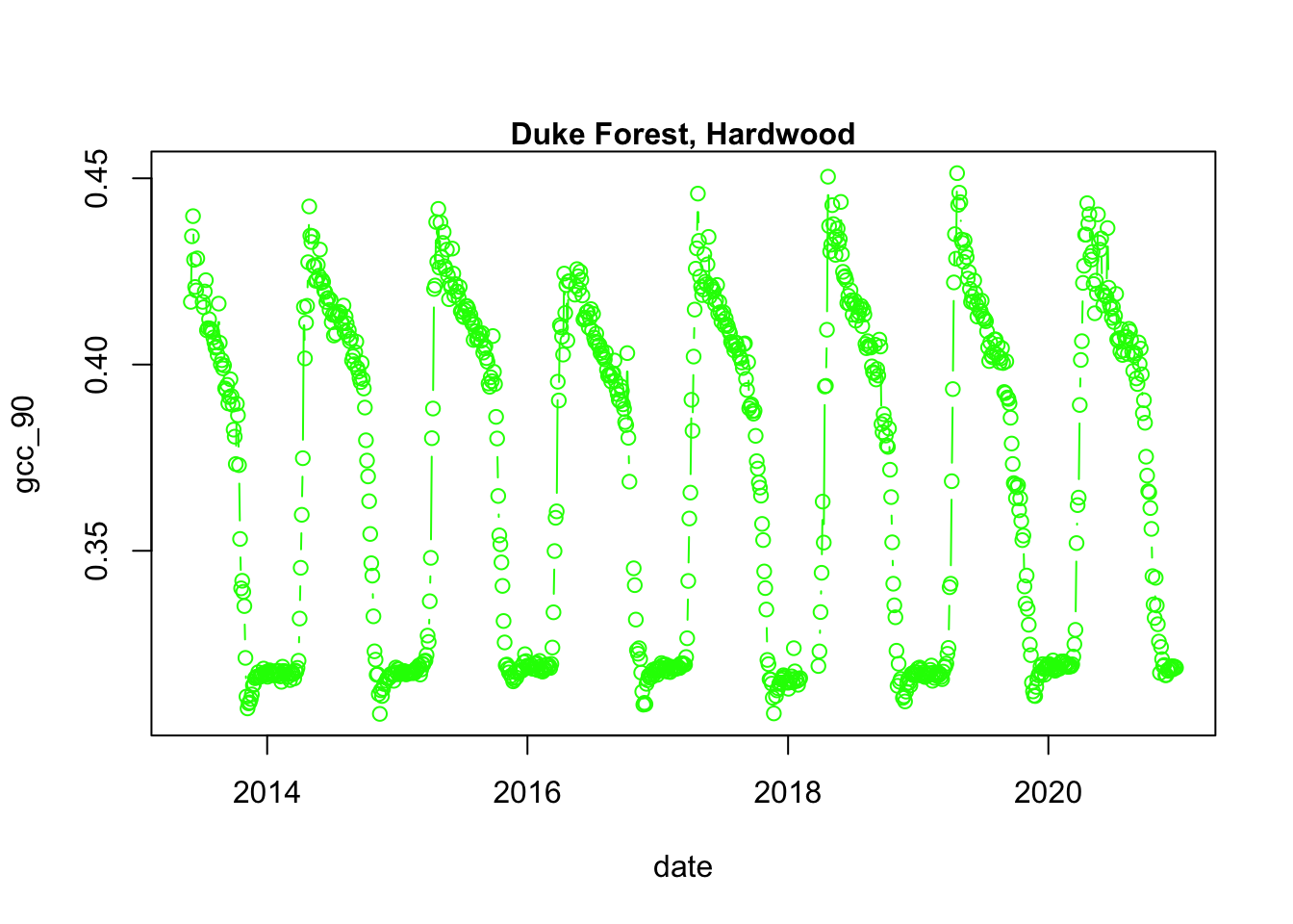
Now, based on either direct API access or via the phenocamapi package, generate a dataframe of phenocam sites. Select two phenocam sites from different plant functional types to explore (e.g. one grassland site and one evergreen needleleaf site)
##         Sitename      Lat        Lon Elev active utc_offset date_first
## 1  archboldbahia 27.16560  -81.21611    8   TRUE         -5 2017-03-21
## 2   arizonagrass 31.59070 -110.50920 1469  FALSE         -7 2008-01-01
## 3       arsgacp2 31.43950  -83.59146  101  FALSE          2 2016-04-27
## 4 bitterbrush001 48.15400 -119.94560  667   TRUE         -8 2020-09-20
## 5        bozeman 45.78306 -110.77778 2332  FALSE         -7 2015-08-16
## 6          butte 45.95304 -112.47964 1682   TRUE         -7 2008-04-01
##    date_last infrared                                              contact1
## 1 2021-02-11        Y      Amartya Saha <asaha AT archbold-station DOT org>
## 2 2010-04-25        N           Mark Heuer <Mark DOT Heuer AT noaa DOT gov>
## 3 2018-01-23        Y David Bosch <David DOT Bosch AT ars DOT usda DOT gov>
## 4 2020-12-29        Y      Brandon Sackmann <bssackmann AT gsi-net DOT com>
## 5 2019-12-18        Y            Paul Stoy <paul DOT stoy AT gmail DOT com>
## 6 2021-02-10        N       James Gallagher <jgallagher AT opendap DOT org>
##                                                     contact2
## 1 Elizabeth Boughton <eboughton AT archbold-station DOT org>
## 2          Tilden Meyers <tilden DOT meyers AT noaa DOT gov>
## 3
## 4            Kenia Whitehead <kwhitehead AT gsi-net DOT com>
## 5
## 6                     Martha Apple <MApple AT mtech DOT edu>
##                                                                        site_description
## 1                                             Archbold Biological Station, Florida, USA
## 2                                                                 Sierra Vista, Arizona
## 3                           Southeast Watershed Research Laboratory EC2 Tifton, Georgia
## 4 Parcel 1 East at Midpoint (Shrub-Steppe - Post Wildfire ca. 2014), Methow, Washington
## 5                                Bangtail Study Area, Montana State University, Montana
## 6                                                    Continental Divide, Butte, Montana
##   site_type                 group camera_description camera_orientation
## 1         I                  LTAR  StarDot NetCam SC                  N
## 2       III                 GEWEX     Olympus D-360L                  N
## 3         I                  LTAR                  N                  N
## 4         I                     N  StarDot NetCam SC                  W
## 5         I AmericaView AMERIFLUX  StarDot NetCam SC                  N
## 6         I              PhenoCam  StarDot NetCam SC                  E
##   flux_data                                          flux_networks
## 1     FALSE                                                   NULL
## 2     FALSE                                                   NULL
## 3     FALSE                                                   NULL
## 4     FALSE                                                   NULL
## 5      TRUE AMERIFLUX, http://ameriflux.lbl.gov, AmeriFlux Network
## 6     FALSE                                                   NULL
##         flux_sitenames
## 1                    N
## 2                    N
## 3                    N
## 4
## 5 US-MTB (forthcoming)
## 6
##                                                                                                                                                                                                                                                                dominant_species
## 1
## 2
## 3
## 4
## 5                                                                                                                                                                                                                                                            Festuca idahoensis
## 6 Agropyron cristatum, Poa pratensis, Phalaris arundinaceae, Carex. sp., Geum triflorum, Ericameria nauseousa, Centaurea macula, Achillea millefolium, Senecio sp., Lupinus sp., Penstemon sp., Linaria vulgaris, Cirsium arvense; Alnus incana, Salix sp., Populus tremuloides
##   primary_veg_type secondary_veg_type site_meteorology MAT_site MAP_site
## 1               GR                  N            FALSE        N        N
## 2               GR                  N            FALSE        N        N
## 3               GR                  N            FALSE        N        N
## 4               GR                 SH            FALSE      8.7      323
## 5               GR                 EN            FALSE        5      850
## 6               GR                 SH            FALSE        N        N
##   MAT_daymet MAP_daymet MAT_worldclim MAP_worldclim koeppen_geiger ecoregion
## 1      22.85       1302          22.5          1208            Cfa         8
## 2      16.25        468          15.3           446            BSk        12
## 3         19       1251          18.7          1213            Cfa         8
## 4       8.35        420           7.3           340            Dsb        10
## 5        2.3        981           0.9           728            Dfb         6
## 6       5.05        365           4.3           311            BSk         6
##   landcover_igbp
## 1             14
## 2              7
## 3             14
## 4              1
## 5             10
## 6             10
##                                                                                                                                                                                                                                                 site_acknowledgements
## 1
## 2
## 3
## 4                                                                                                                                                                 Research at this site is supported by GSI Environmental Inc. (http://www.gsi-net.com), Olympia, WA.
## 5 Research at the Bozeman site is supported by Colorado State University and the AmericaView program (grants G13AC00393, G11AC20461, G15AC00056) with phenocam equipment and deployment sponsored by the Department of Interior North Central Climate Science Center.
## 6                                                         Research at the Continental Divide PhenoCam Site in Butte, Montana is supported by the National Science Foundation-EPSCoR (grant NSF-0701906), OpenDap, Inc., and Montana Tech of the University of Montana
##                           modified
## 1 2019-01-07T18:36:07.631244-05:00
## 2 2018-04-13T10:46:23.462958-04:00
## 3 2018-06-18T20:27:17.280524-04:00
## 4 2020-10-30T10:48:53.990761-04:00
## 5 2016-11-01T15:42:19.771057-04:00
## 6 2016-11-01T15:42:19.846100-04:00## Sitename Lat Lon Elev active utc_offset date_first date_last
## 5 bozeman 45.78306 -110.7778 2332 FALSE -7 2015-08-16 2019-12-18
## infrared contact1 contact2
## 5 Y Paul Stoy <paul DOT stoy AT gmail DOT com>
## site_description site_type
## 5 Bangtail Study Area, Montana State University, Montana I
## group camera_description camera_orientation flux_data
## 5 AmericaView AMERIFLUX StarDot NetCam SC N TRUE
## flux_networks flux_sitenames
## 5 AMERIFLUX, http://ameriflux.lbl.gov, AmeriFlux Network US-MTB (forthcoming)
## dominant_species primary_veg_type secondary_veg_type site_meteorology
## 5 Festuca idahoensis GR EN FALSE
## MAT_site MAP_site MAT_daymet MAP_daymet MAT_worldclim MAP_worldclim
## 5 5 850 2.3 981 0.9 728
## koeppen_geiger ecoregion landcover_igbp
## 5 Dfb 6 10
## site_acknowledgements
## 5 Research at the Bozeman site is supported by Colorado State University and the AmericaView program (grants G13AC00393, G11AC20461, G15AC00056) with phenocam equipment and deployment sponsored by the Department of Interior North Central Climate Science Center.
## modified
## 5 2016-11-01T15:42:19.771057-04:00Chose your own sites and build out your code chunk here:
## [1] "build your code here"Koen Huffkens developed the phenocamr package, which streamlines access to quality controlled data. We will now use this package to download and process site based data according to a standardized methodology.
A full description of the methodology is provided in Scientific Data: Tracking vegetation phenology across diverse North American biomes using PhenoCam imagery (Richardson et al. 2018).
#uncomment if you need to install via devtools
#if(!require(devtools)){install.package(devtools)}
#devtools::install_github("khufkens/phenocamr")
library(phenocamr)
Use the dataframe of sites that you want to analyze to feed the phenocamr package. Note: you can choose either a 1 or 3 day product
dir.create('data/', showWarnings = F)

phenocamr::download_phenocam(
  frequency = 3,
  veg_type = 'DB',
  roi_id = 1000,
  site = 'harvard',
  phenophase = TRUE,
  out_dir = "data/"
)
## Downloading: harvard_DB_1000_3day.csv## -- Flagging outliers!## -- Smoothing time series!## -- Estimating transition dates!## Downloading: harvardbarn_DB_1000_3day.csv## -- Flagging outliers!## -- Smoothing time series!## -- Estimating transition dates!## Downloading: harvardbarn2_DB_1000_3day.csv## -- Flagging outliers!## -- Smoothing time series!## -- Estimating transition dates!## Downloading: harvardfarmsouth_DB_1000_3day.csv## -- Flagging outliers!## -- Smoothing time series!## -- Estimating transition dates!## Downloading: harvardhemlock_DB_1000_3day.csv## -- Flagging outliers!## -- Smoothing time series!## -- Estimating transition dates!## Downloading: harvardlph_DB_1000_3day.csv## -- Flagging outliers!## -- Smoothing time series!## -- Estimating transition dates!#> Downloading: harvard_DB_1000_3day.csv
#> -- Flagging outliers!
#> -- Smoothing time series!
#> -- Estimating transition dates!Now look in your working directory. You have data! Read it in:
# load the time series data but replace the csv filename with whatever you downloaded
df <- read.table("data/harvard_DB_1000_3day.csv", header = TRUE, sep = ",")

# read in the transition date file
td <- read.table("data/harvard_DB_1000_3day_transition_dates.csv",
                header = TRUE,
                sep = ",")
Let’s take a look at the data:
p = plot_ly() %>%
  add_trace(
    data = df,
    x = ~ as.Date(date),
    y = ~ smooth_gcc_90,
    name = 'Smoothed GCC',
    showlegend = TRUE,
    type = 'scatter',
    mode = 'line'
  ) %>% add_markers(
    data=df,
    x ~ as.Date(date),
    y = ~gcc_90,
    name = 'GCC',
    type = 'scatter',
    color ='#07A4B5',
    opacity=.5
  )
p
## Warning: `arrange_()` is deprecated as of dplyr 0.7.0.
## Please use `arrange()` instead.
## See vignette('programming') for more help
## This warning is displayed once every 8 hours.
## Call `lifecycle::last_warnings()` to see where this warning was generated.## Warning: Ignoring 3319 observations## Warning in RColorBrewer::brewer.pal(N, "Set2"): minimal value for n is 3, returning requested palette with 3 different levels
## Warning in RColorBrewer::brewer.pal(N, "Set2"): minimal value for n is 3, returning requested palette with 3 different levelsWhat patterns do you notice? How would we go about determining say the start of spring? (SOS)
4.12.4 Threshold values
Let’s subset the transition date (td) for each year when 25% of the greenness amplitude (of the 90^th) percentile is reached (threshold_25).
# select the rising (spring dates) for 25% threshold of Gcc 90
spring <- td[td$direction == "rising" & td$gcc_value == "gcc_90",]
Let’s create a simple plot_ly line graph of the smooth Green Chromatic Coordinate (Gcc) and add points for transition dates:
p = plot_ly() %>%
  add_trace(
    data = df,
    x = ~ as.Date(date),
    y = ~ smooth_gcc_90,
    name = 'PhenoCam GCC',
    showlegend = TRUE,
    type = 'scatter',
    mode = 'line'
  ) %>% add_markers(
    data= spring,
    x = ~ as.Date(spring$transition_25, origin = "1970-01-01"),
    y = ~ spring$threshold_25,
    type = 'scatter',
    mode = 'marker',
    name = 'Spring Dates')

pHowever, if you want more control over the parameters used during processing, you can run through the three default processing steps as implemented in download_phenocam() and set parameters manually.
Of particular interest is the option to specify your own threshold used in determining transition dates.
What would be a reasonable threshold for peak greenness? Or autumn onset? Look at the ts dataset and phenocamr package and come up with a threshold. Use the same code to plot it here:
# #some hint code
# #what does 'rising' versus 'falling' denote?
# #what threshold should you choose?
# #td <- phenophases("butte_GR_1000_3day.csv",
# #            internal = TRUE,
# #            upper_thresh = 0.8)
fall <- td[td$direction == "falling" & td$gcc_value == "gcc_90",]
#Now generate a fall dataframe, what metrics should you use?
4.12.5 Comparing phenology across vegetation types
Let’s load in a function to make plotting smoother. I’ve dropped it here in the markdown so that you can edit it and re-run it as you see fit:
gcc_plot = function(gcc, spring, fall){
  unix = "1970-01-01"

  p = plot_ly(
    data = gcc,
    x = ~ date,
    y = ~ gcc_90,
    showlegend = FALSE,
    type = 'scatter',
    mode = 'line'
  ) %>%
    add_trace(
      y = ~ smooth_gcc_90,
      mode = "lines",
      line = list(width = 2, color = "rgb(120,120,120)"),
      name = "Gcc loess fit",
      showlegend = TRUE
    ) %>%
    # SOS spring
    # 10%
    add_trace(
      data = spring,
      x = ~ as.Date(transition_10),
      y = ~ threshold_10,
      mode = "markers",
      type = "scatter",
      marker = list(color = "#7FFF00", symbol = "circle"),
      name = "SOS (10%)",
      showlegend = TRUE
    ) %>%
    add_segments(x = ~ as.Date(transition_10_lower_ci),
                 xend = ~ as.Date(transition_10_upper_ci),
                 # y = ~ 0,
                 # yend = ~ 1,
                 y = ~ threshold_10,
                 yend = ~ threshold_10,
                 line = list(color = "#7FFF00"),
                 name = "SOS (10%) - CI"
    ) %>%
    # 25 %
    add_trace(
      x = ~ as.Date(transition_25),
      y = ~ threshold_25,
      mode = "markers",
      type = "scatter",
      marker = list(color = "#66CD00", symbol = "square"),
      showlegend = TRUE,
      name = "SOS (25%)"
    ) %>%
    add_segments(x = ~ as.Date(transition_25_lower_ci),
                 xend = ~ as.Date(transition_25_upper_ci),
                 y = ~ threshold_25,
                 yend = ~ threshold_25,
                 line = list(color = "#66CD00"),
                 name = "SOS (25%) - CI"
    ) %>%
    # 50 %
    add_trace(
      x = ~ as.Date(transition_50),
      y = ~ threshold_50,
      mode = "markers",
      type = "scatter",
      marker = list(color = "#458B00", symbol = "diamond"),
      showlegend = TRUE,
      name = "SOS (50%)"
    ) %>%
    add_segments(x = ~ as.Date(transition_50_lower_ci),
                 xend = ~ as.Date(transition_50_upper_ci),
                 y = ~ threshold_50,
                 yend = ~ threshold_50,
                 line = list(color = "#458B00"),
                 name = "SOS (50%) - CI"
    ) %>%

    # EOS fall
    # 50%
    add_trace(
      data = fall,
      x = ~ as.Date(transition_50),
      y = ~ threshold_50,
      mode = "markers",
      type = "scatter",
      marker = list(color = "#FFB90F", symbol = "diamond"),
      showlegend = TRUE,
      name = "EOS (50%)"
    ) %>%
    add_segments(x = ~ as.Date(transition_50_lower_ci),
                 xend = ~ as.Date(transition_50_upper_ci),
                 y = ~ threshold_50,
                 yend = ~ threshold_50,
                 line = list(color = "#FFB90F"),
                 name = "EOS (50%) - CI"
    ) %>%
    # 25 %
    add_trace(
      x = ~ as.Date(transition_25),
      y = ~ threshold_25,
      mode = "markers",
      type = "scatter",
      marker = list(color = "#CD950C", symbol = "square"),
      showlegend = TRUE,
      name = "EOS (25%)"
    ) %>%
    add_segments(x = ~ as.Date(transition_25_lower_ci),
                 xend = ~ as.Date(transition_25_upper_ci),
                 y = ~ threshold_25,
                 yend = ~ threshold_25,
                 line = list(color = "#CD950C"),
                 name = "EOS (25%) - CI"
    ) %>%
    # 10 %
    add_trace(
      x = ~ as.Date(transition_10),
      y = ~ threshold_10,
      mode = "markers",
      marker = list(color = "#8B6508", symbol = "circle"),
      showlegend = TRUE,
      name = "EOS (10%)"
    ) %>%
    add_segments(x = ~ as.Date(transition_10_lower_ci),
                 xend = ~ as.Date(transition_10_upper_ci),
                 y = ~ threshold_10,
                 yend = ~ threshold_10,
                 line = list(color = "#8B6508"),
                 name = "EOS (10%) - CI"
    )
  return (p)
}
gcc_p = gcc_plot(df, spring, fall)
gcc_p <- gcc_p %>%
layout(
legend = list(x = 0.9, y = 0.9),
xaxis = list(
type = 'date',
tickformat = " %B<br>%Y",
title='Year'),
yaxis = list(
title = 'PhenoCam GCC'
))
gcc_p## Warning: Ignoring 3319 observations## Warning: `group_by_()` is deprecated as of dplyr 0.7.0.
## Please use `group_by()` instead.
## See vignette('programming') for more help
## This warning is displayed once every 8 hours.
## Call `lifecycle::last_warnings()` to see where this warning was generated.## Warning: Can't display both discrete & non-discrete data on same axisWhat is the difference in 25% greenness onset for your first site? #hint, look at the spring dataframe you just generated
#more code hints
# dates_split <- data.frame(date = d,
#                  year = as.numeric(format(d, format = "%Y")),
#                  month = as.numeric(format(d, format = "%m")),
#                  day = as.numeric(format(d, format = "%d")))
Generate a plot of smoothed gcc and transition dates for your two sites and subplot them. What do you notice?
4.12.6 In Class Hands-on Coding: Comparing phenology of the same plant function type (PFT) across climate space
As Dr. Richardson mentioned in his introduction lecture, the same plant functional types (e.g. grasslands) can have very different phenologogical cycles. Let’s pick two phenocam grassland sites: one from a tropical climate (kamuela), and one from an arid climate (konza):
Now pull data for those sites via phenocamr or the phenocamapi
## [1] "code here"Now let’s create a subplot of your grasslands to compare phenology, some hint code below:
Once you have a subplot of grassland phenology across 2 climates answer the following questions in your markdown: 1. What seasonal patterns do you see? 2. Do you think you set your thresholds correctly for transition dates/phenophases? How might that very as a function of climate? 3. What are the challenges of forecasting or modeling tropical versus arid grasslands?
4.13 Digital Repeat Photography Coding Lab
4.13.1 Quantifying haze and redness to evaluate California wildfires
Pull mid-day imagery for September 1-7th, 2019 and 2020 for the canopy-level camera
NEON.D17.SOAP.DP1.00033. Create a 2-panel plot showing those images in 2019 (left) and 2020 (right).Use the
hazeRpackage to quantify the haze in each of those images. Print a summary of your results.Generate a density function RGB plot for your haziest image in 2020, and one for the same date in 2019. Create a 2-panel plot showing 2019 on the left and 2020 on the right.
Pull timesseries data via the
phenocamapipackage. Calculate the difference in the rcc90 between 2019 and 2020 over the same time period as your images.Create a summary plot showing haze as a bar and the differenece in rcc90 from question 4 as a timersies.
Answer the following questions:
Does the
hazeRpackage pick up smokey images?If you were to use color coordinates, which color band would be most useful to highlight smoke and why?
Optional Bonus Points:
Repeat the above calculations for the understory camera on the same tower NEON.D17.SOAP.DP1.00042 and produce the same plots. Which camera is ‘better’ and capturing wildfire? Why do you think that is so?
4.14 PhenoCam Culmination Activity
Write up a 1-page summary of a project that you might want to explore using PhenoCam data over the duration of this course. Include the types of PhenoCam (and other data) that you will need to implement this project. Save this summary as you will be refining and adding to your ideas over the course of the semester.